In Chapter 1, An Introduction to Query Tuning and Optimization, we introduced you to reading execution plans as the primary tool we’ll use to interact with the SQL Server query processor. We also checked out the SET STATISTICS TIME and SET STATISTICS IO statements, which can provide you with additional performance information about your queries. In this chapter, we continue where we left off in the previous chapter. We will look into additional tuning tools and techniques you can use to find out how many server resources your queries are using and how to find the most expensive queries on your system.

Dynamic management views (DMVs) were introduced with SQL Server 2005 as a great tool to diagnose problems, tune performance, and monitor the health of a SQL Server instance. There are many DMVs available, and the first section in this chapter focuses on sys.dm_exec_requests, sys.dm_exec_sessions, and sys.dm_exec_query_stats, which you can use to find out the server resources, such as CPU and I/O, that are used by queries running on the system. Many more DMVs will be introduced in other chapters of this book, including later in this chapter, when we cover extended events.

Although SQL Trace has been deprecated as of SQL Server 2012, it’s still widely used and will be available in some of the next versions of SQL Server. SQL Trace is usually related to SQL Server Profiler because using this tool is the easiest way to define and run a trace, and it is also the tool of choice for scripting and creating a server trace, which is used in some scenarios where running Profiler directly may be expensive. In this chapter, we’ll cover some of the trace events we would be more interested in when tracing query execution for performance problems.

Following on from the same concept as SQL Trace, in the next section, we will explore extended events. All the basic concepts and definitions will be explained first, including events, predicates, actions, targets, and sessions. Then, we will create some sessions to obtain performance information about queries. Because most SQL Server professionals are already familiar with SQL Trace or Profiler, we will also learn how to map the old trace events to the new extended events.

Finally, the Data Collector, a feature introduced with SQL Server 2008, will be shown as a tool that can help you proactively collect performance data that can be used to troubleshoot performance problems when they occur.

In this chapter, we will cover the following topics:

• DMVs and DMFs
• SQL Trace
• Extended events
• The Data Collector

In this section, we will show you several dynamic management views (DMVs) and dynamic management functions (DMFs) that can help you to find out the number of server resources that are being used by your queries and to find the most expensive queries in your SQL Server instance.

sys.dm_exec_requests and sys.dm_exec_sessions

The sys.dm_exec_requests DMV can be used to display the requests currently executing on SQL Server, whereas sys.dm_exec_sessions shows the authenticated sessions on the instance. Although these DMVs include many columns, in this section, we will focus on the ones related to resource usage and query performance. You can look at the definitions of the other columns on the SQL Server documentation.

Both DMVs share several columns, as shown in the following table:

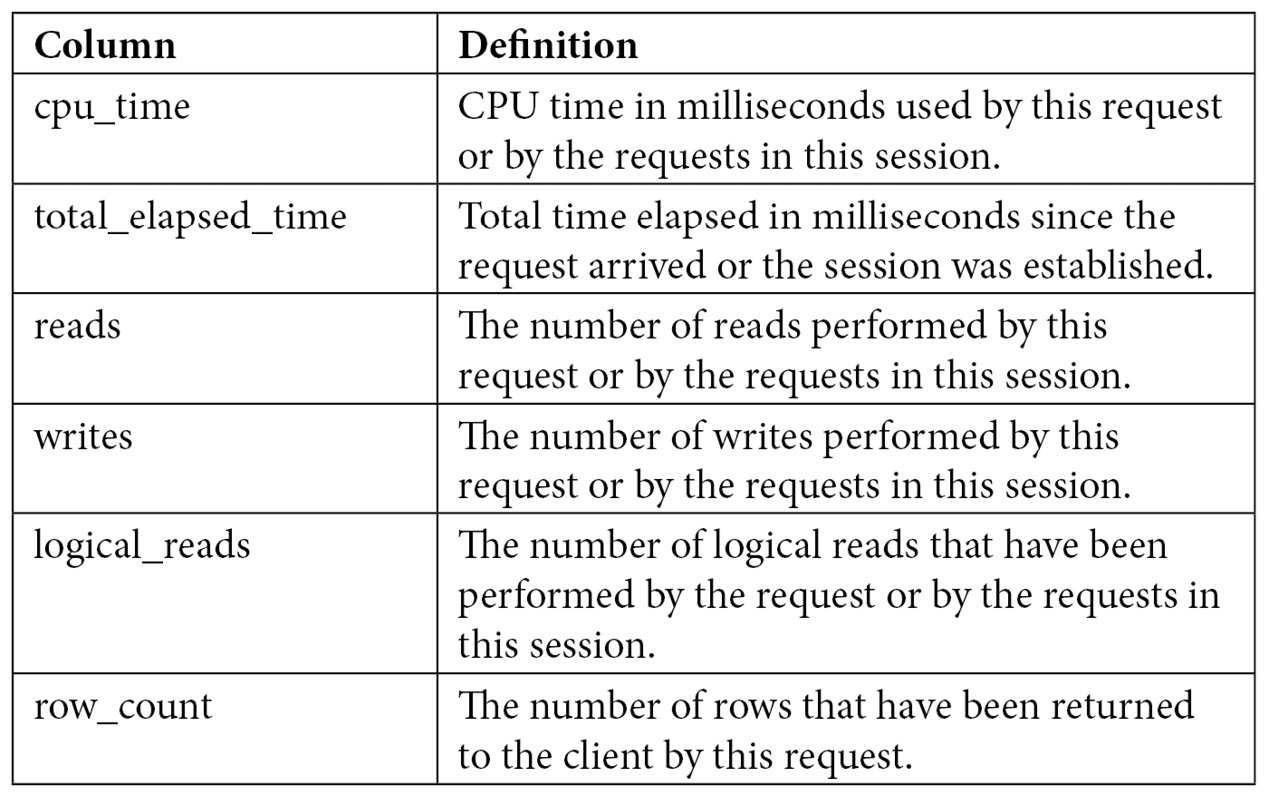
Table 2.1 – The sys.dm_exec_requests and sys.dm_exec_sessions columns

sys.dm_exec_requests will show the resources that are used by a specific request currently executing, whereas sys.dm_exec_sessions will show the accumulated resources of all the requests completed by a session. To understand how these two DMVs collect resource usage information, we can use a query that takes at least a few seconds. Open a new query in Management Studio and get its session ID (for example, using SELECT @@SPID), but make sure you don’t run anything on it yet – the resource usage will be accumulated on the sys.dm_exec_sessions DMV. Copy and be ready to run the following code on that window:

DBCC FREEPROCCACHE
DBCC DROPCLEANBUFFERS
GO
SELECT * FROM Production.Product p1 CROSS JOIN Production.Product p2

Copy the following code to a second window, replacing session_id with the value you obtained in the first window:

SELECT cpu_time, reads, total_elapsed_time, logical_reads, row_count
FROM sys.dm_exec_requests
WHERE session_id = 56
GO
SELECT cpu_time, reads, total_elapsed_time, logical_reads, row_count
FROM sys.dm_exec_sessions
WHERE session_id = 56

Run the query on the first session and, at the same time, run the code on the second session several times to see the resources used. The following output shows a sample execution while the query is still running and has not been completed yet. Notice that the sys.dm_exec_requests DMV shows the partially used resources and that sys.dm_exec_sessions shows no used resources yet. Most likely, you will not see the same results for sys.dm_exec_requests:

After the query completes, the original request no longer exists and sys.dm_exec_requests returns no data at all. sys.dm_exec_sessions now records the resources used by the first query:

If you run the query on the first session again, sys.dm_exec_sessions will accumulate the resources used by both executions, so the values of the results will be slightly more than twice their previous values, as shown here:

Keep in mind that CPU time and duration may vary slightly during different executions and that you will likely get different values as well. The number of reads for this execution is 8,192, and we can see the accumulated value of 16,384 for two executions. In addition, the sys.dm_exec_requests DMV only shows information of currently executing queries, so you may not see this particular data if a query completes before you can query it.

In summary, sys.dm_exec_requests and sys.dm_exec_sessions are useful for inspecting the resources being used by a request or the accumulation of resources being used by requests on a session since its creation.

Sys.dm_exec_query_stats

If you’ve ever worked with any version of SQL Server older than SQL Server 2005, you may remember how difficult it was to find the most expensive queries in your instance. Performing that kind of analysis usually required running a server trace in your instance for some time and then analyzing the collected data, usually in the size of gigabytes, using third-party tools or your own created methods (a very time-consuming process). Not to mention the fact that running such a trace could also affect the performance of a system, which most likely is having a performance problem already.

DMVs were introduced with SQL Server 2005 and are a great help to diagnose problems, tune performance, and monitor the health of a server instance. In particular, sys.dm_exec_query_stats provides a rich amount of information not available before in SQL Server regarding aggregated performance statistics for cached query plans. This information helps you avoid the need to run a trace, as mentioned earlier, in most cases. This view returns a row for each statement available in the plan cache, and SQL Server 2008 added enhancements such as the query hash and plan hash values, which will be explained shortly.

Let’s take a quick look at understanding how sys.dm_exec_query_stats works and the information it provides. Create the following stored procedure with three simple queries:

CREATE PROC test
AS
SELECT * FROM Sales.SalesOrderDetail WHERE SalesOrderID = 60677
SELECT * FROM Person.Address WHERE AddressID = 21
SELECT * FROM HumanResources.Employee WHERE BusinessEntityID = 229

Run the following code to clean the plan cache (so that it is easier to inspect), remove all the clean buffers from the buffer pool, execute the created test stored procedure, and inspect the plan cache. Note that the code uses the sys.dm_exec_sql_text DMF, which requires a sql_handle or plan_handle value and returns the text of the SQL batch:

DBCC FREEPROCCACHE
DBCC DROPCLEANBUFFERS
GO
EXEC test
GO
SELECT * FROM sys.dm_exec_query_stats
CROSS APPLY sys.dm_exec_sql_text(sql_handle)
WHERE objectid = OBJECT_ID('dbo.test')

Examine the output. Because the number of columns is too large to show in this book, only some of the columns are shown here:

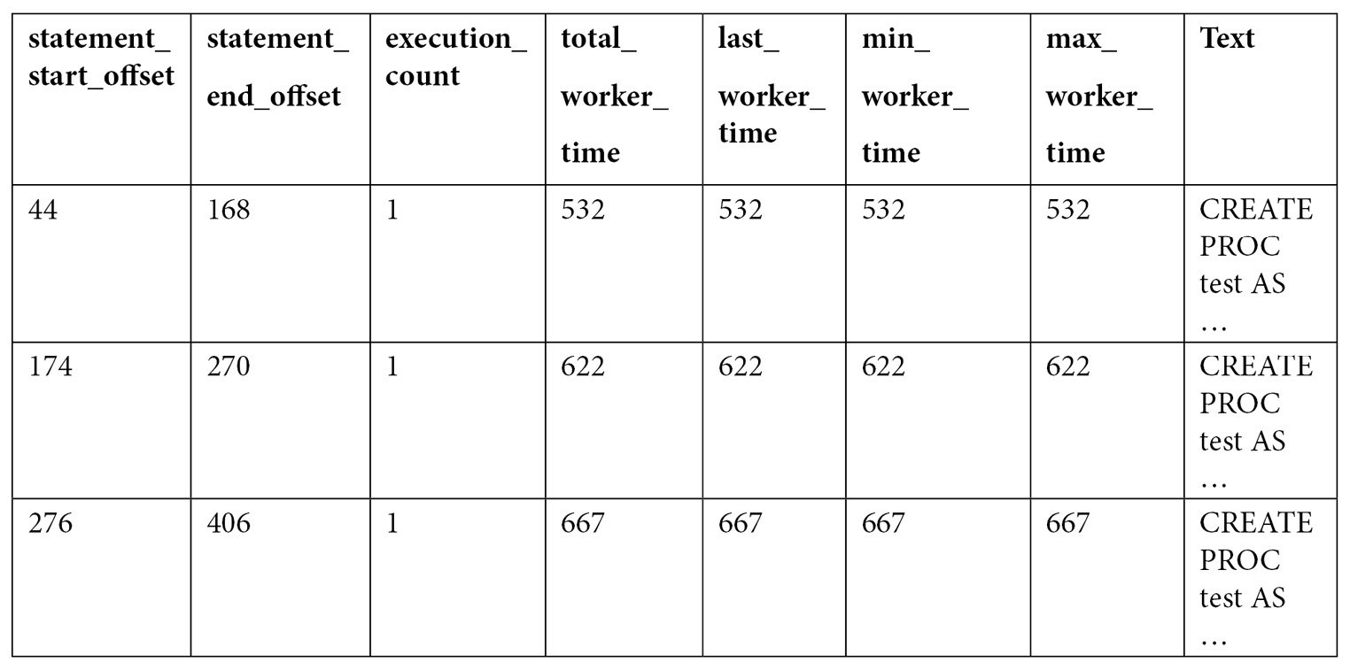
As you can see by looking at the query text, all three queries were compiled as part of the same batch, which we can also verify by validating they have the same plan_handle and sql_handle. statement_start_offset and statement_end_offset can be used to identify the particular queries in the batch, a process that will be explained later in this section. You can also see the number of times the query was executed and several columns showing the CPU time used by each query, such as total_worker_time, last_worker_time, min_worker_time, and max_worker_time. Should the query be executed more than once, the statistics would show the accumulated CPU time on total_worker_time. Not shown in the previous output are additional performance statistics for physical reads, logical writes, logical reads, CLR time, and elapsed time. The following table shows the list of columns, including performance statistics and their documented description:

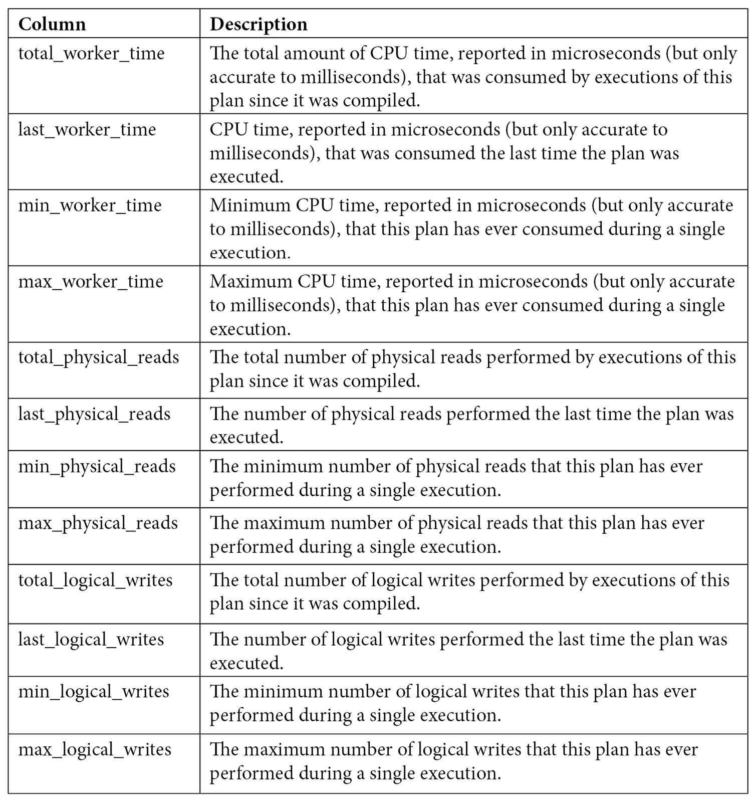
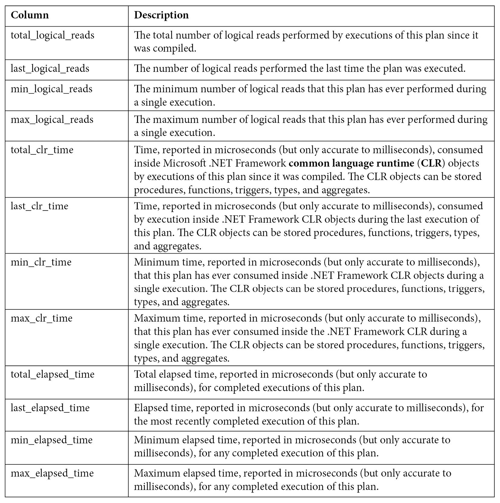
Table 2.2 – The sys.dm_exec_query_stats columns

Keep in mind that this view only shows statistics for completed query executions. You can look at sys.dm_exec_requests, as explained earlier, for information about queries currently executing. Finally, as explained in the previous chapter, certain types of execution plans may never be cached, and some cached plans may also be removed from the plan cache for several reasons, including internal or external memory pressure on the plan cache. Information for these plans will not be available on sys.dm_exec_query_stats.

Now, let’s look at the statement_start_offset and statement_end_offset values.

Understanding statement_start_offset and statement_end_offset

As shown from the previous output of sys.dm_exec_query_stats, the sql_handle, plan_handle, and text columns showing the code for the stored procedure are the same in all three records. The same plan and query are used for the entire batch. So, how do we identify each of the SQL statements, for example, supposing that only one of them is expensive? We must use the statement_start_offset and statement_end_offset columns. statement_start_offset is defined as the starting position of the query that the row describes within the text of its batch, whereas statement_end_offset is the ending position of the query that the row describes within the text of its batch. Both statement_start_offset and statement_end_offset are indicated in bytes, starting with 0. A value of –1 indicates the end of the batch.

We can easily extend our previous query to inspect the plan cache to use statement_start_offset and statement_end_offset and get something like the following:

DBCC FREEPROCCACHE
DBCC DROPCLEANBUFFERS
GO
EXEC test
GO
SELECT SUBSTRING(text, (statement_start_offset/2) + 1,
((CASE statement_end_offset
WHEN -1
THEN DATALENGTH(text)
ELSE
statement_end_offset
END
- statement_start_offset)/2) + 1) AS statement_text, *
FROM sys.dm_exec_query_stats
CROSS APPLY sys.dm_exec_sql_text(sql_handle)
WHERE objectid = OBJECT_ID('dbo.test')

This would produce output similar to the following (only a few columns are shown here):

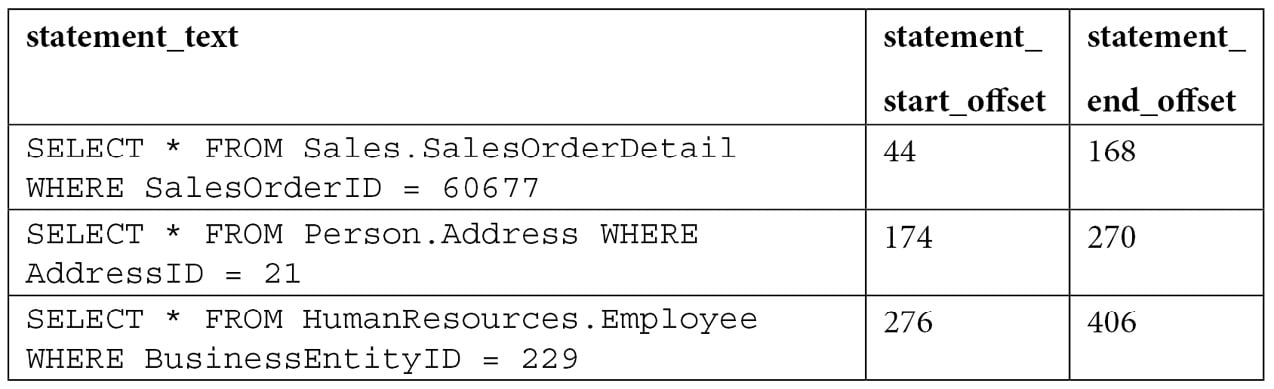
The query makes use of the SUBSTRING function, as well as statement_start_offset and statement_end_offset values, to obtain the text of the query within the batch. Division by 2 is required because the text data is stored as Unicode.

To test the concept for a particular query, you can replace the values for statement_start_offset and statement_end_offset directly for the first statement (44 and 168, respectively) and provide sql_handle or plan_handle, (returned in the previous query and not printed in the book) as shown here, to get the first statement that was returned:

SELECT SUBSTRING(text, 44 / 2 + 1, (168 - 44) / 2 + 1) FROM sys.dm_exec_sql_text(0x03000500996DB224E0B27201B7A1000001000000000000 000000000000000000000000000000000000000000)

sql_handle and plan_handle

The sql_handle value is a hash value that refers to the batch or stored procedure the query is part of. It can be used in the sys.dm_exec_sql_text DMF to retrieve the text of the query, as demonstrated previously. Let’s use the example we used previously:

SELECT * from sys.dm_exec_sql_text(0x03000500996DB224E0B27201B7A1000001000000 000000000000000000000000000000000000000000000000)

We would get the following in return:

The sql_handle hash is guaranteed to be unique for every batch in the system. The text of the batch is stored in the SQL Manager Cache or SQLMGR, which you can inspect by running the following query:

SELECT * FROM sys.dm_os_memory_objects
WHERE type = 'MEMOBJ_SQLMGR'

Because a sql_handle has a 1:N relationship with a plan_handle (that is, there can be more than one generated executed plan for a particular query), the text of the batch will remain on the SQLMGR cache store until the last of the generated plans is evicted from the plan cache.

The plan_handle value is a hash value that refers to the execution plan the query is part of and can be used in the sys.dm_exec_query_plan DMF to retrieve such an execution plan. It is guaranteed to be unique for every batch in the system and will remain the same, even if one or more statements in the batch are recompiled. Here is an example:

SELECT * FROM sys.dm_exec_query_plan(0x05000500996DB224B0C9B8F8010000000100 0000000000000000000000000000000000000000000000000000)

Running the preceding code will return the following output, and clicking the query_plan link will display the requested graphical execution plan. Again, make sure you are using a valid plan_handle value:

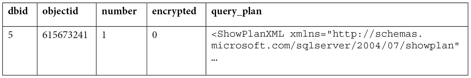
Cached execution plans are stored in the SQLCP and OBJCP cache stores: object plans, including stored procedures, triggers, and functions, are stored in the OBJCP cache store, whereas plans for ad hoc, auto parameterized, and prepared queries are stored in the SQLCP cache store.

query_hash and plan_hash

Although sys.dm_exec_query_stats was a great resource that provided performance statistics for cached query plans when it was introduced in SQL Server 2005, one of its limitations was that it was not easy to aggregate the information for the same query when this query was not parameterized. The query_hash and plan_hash columns, introduced with SQL Server 2008, provide a solution to this problem. To understand the problem, let’s look at an example of the behavior of sys.dm_exec_query_stats when a query is auto-parameterized:

DBCC FREEPROCCACHE
DBCC DROPCLEANBUFFERS
GO
SELECT * FROM Person.Address
WHERE AddressID = 12
GO
SELECT * FROM Person.Address
WHERE AddressID = 37
GO
SELECT * FROM sys.dm_exec_query_stats

Because AddressID is part of a unique index, the AddressID = 12 predicate would always return a maximum of one record, so it is safe for the query optimizer to auto-parameterize the query and use the same plan. Here is the output:

In this case, we only have one plan that’s been reused for the second execution, as shown in the execution_count value. Therefore, we can also see that plan reuse is another benefit of parameterized queries. However, we can see a different behavior by running the following query:

DBCC FREEPROCCACHE
DBCC DROPCLEANBUFFERS
GO
SELECT * FROM Person.Address
WHERE StateProvinceID = 79
GO
SELECT * FROM Person.Address
WHERE StateProvinceID = 59
GO
SELECT * FROM sys.dm_exec_query_stats

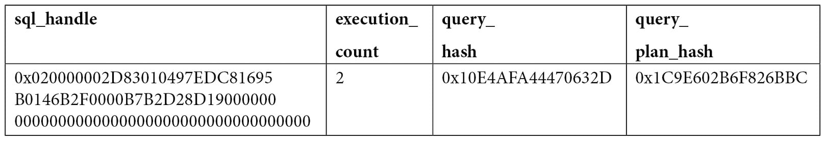
Because a filter with an equality comparison on StateProvinceID could return zero, one, or more values, it is not considered safe for SQL Server to auto-parameterize the query; in fact, both executions return different execution plans. Here is the output:

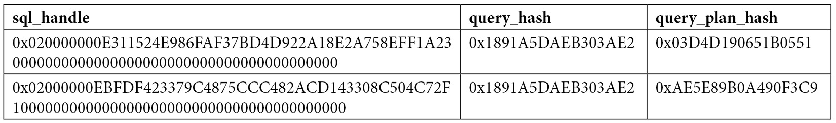
As you can see, sql_handle, plan_handle (not shown), and query_plan_hash have different values because the generated plans are different. However, query_hash is the same because it is the same query, only with a different parameter. Supposing that this was the most expensive query in the system and there are multiple executions with different parameters, it would be very difficult to find out that all those execution plans do belong to the same query. This is where query_hash can help. You can use query_hash to aggregate performance statistics of similar queries that are not explicitly or implicitly parameterized. Both query_hash and plan_hash are available on the sys.dm_exec_query_stats and sys.dm_exec_requests DMVs.

The query_hash value is calculated from the tree of logical operators that was created after parsing just before query optimization. This logical tree is used as the input to the query optimizer. Because of this, two or more queries do not need to have the same text to produce the same query_hash value since parameters, comments, and some other minor differences are not considered. And, as shown in the first example, two queries with the same query_hash value can have different execution plans (that is, different query_plan_hash values). On the other hand, query_plan_hash is calculated from the tree of physical operators that makes up an execution plan. If two plans are the same, although very minor differences are not considered, they will produce the same plan hash value as well.

Finally, a limitation of the hashing algorithms is that they can cause collisions, but the probability of this happening is extremely low. This means that two similar queries may produce different query_hash values or that two different queries may produce the same query_hash value, but again, the probability of this happening is extremely low, and it should not be a concern.

Finding expensive queries

Now, let’s apply some of the concepts explained in this section and use the sys.dm_exec_query_stats DMV to find the most expensive queries in your system. A typical query to find the most expensive queries on the plan cache based on CPU is shown in the following code. Note that the query is grouped on the query_hash value to aggregate similar queries, regardless of whether or not they are parameterized:

SELECT TOP 20 query_stats.query_hash,
SUM(query_stats.total_worker_time) / SUM(query_stats.execution_count)
AS avg_cpu_time,
MIN(query_stats.statement_text) AS statement_text
FROM
(SELECT qs.*,
SUBSTRING(st.text, (qs.statement_start_offset/2) + 1,
 ((CASE statement_end_offset
WHEN -1 THEN DATALENGTH(ST.text)
ELSE qs.statement_end_offset END
- qs.statement_start_offset)/2) + 1) AS statement_text
FROM sys.dm_exec_query_stats qs
CROSS APPLY sys.dm_exec_sql_text(qs.sql_handle) AS st) AS query_stats
GROUP BY query_stats.query_hash
ORDER BY avg_cpu_time DESC

You may also notice that each returned row represents a query in a batch (for example, a batch with five queries would have five records on the sys.dm_exec_query_stats DMV, as explained earlier). We could trim the previous query into something like the following query to focus on the batch and plan level instead. Notice that there is no need to use the statement_start_offset and statement_end_offset columns to separate the particular queries and that this time, we are grouping on the query_plan_hash value:

SELECT TOP 20 query_plan_hash,
SUM(total_worker_time) / SUM(execution_count) AS avg_cpu_time,
MIN(plan_handle) AS plan_handle, MIN(text) AS query_text
FROM sys.dm_exec_query_stats qs
CROSS APPLY sys.dm_exec_sql_text(qs.plan_handle) AS st
GROUP BY query_plan_hash
ORDER BY avg_cpu_time DESC

These examples are based on CPU time (worker time). Therefore, in the same way, you can update these queries to look for other resources listed on sys.dm_exec_query_stats, such as physical reads, logical writes, logical reads, CLR time, and elapsed time.

Finally, we could also apply the same concept to find the most expensive queries that are currently executing, based on sys.dm_exec_requests, as shown in the following query:

SELECT TOP 20 SUBSTRING(st.text, (er.statement_start_offset/2) + 1,
((CASE statement_end_offset
WHEN -1
THEN DATALENGTH(st.text)
ELSE
er.statement_end_offset
END
- er.statement_start_offset)/2) + 1) AS statement_text
, *
FROM sys.dm_exec_requests er
CROSS APPLY sys.dm_exec_sql_text(er.sql_handle) st
ORDER BY total_elapsed_time DESC

Blocking and waits

We have talked about queries using resources such as CPU, memory, or disk and measured as CPU time, logical reads, and physical reads, among other performance counters. In SQL Server, however, those resources may not available immediately and your queries may have to wait until they are, causing delays and other performance problems. Although those waits are expected and could be unnoticeable, in some cases, this could be unacceptable, requiring additional troubleshooting. SQL Server provides several ways to track these waits, including several DMVs, which we will cover next, or the WaitsStat element, which we covered in Chapter 1, An Introduction to Query Tuning and Optimization.

Blocking can be seen as a type of wait and occurs all the time on relational databases, as it is required for applications to correctly access and change data. But its duration should be unnoticeable and should not impact applications. So, similar to most other wait types, excessive blocking could be a common performance problem too.

Finally, there are some wait types that, even in large wait times, never impact the performance of some other queries. A few examples of such wait types are LAZYWRITER_SLEEP, LOGMGR_QUEUE, and DIRTY_PAGE_POOL and they are typically filtered out when collecting wait information.

Let me show you a very simple example of blocking so that you can understand how to detect it and troubleshoot it. Using the default isolation level, which is read committed, the following code will block any operation trying to access the same data:

BEGIN TRANSACTION
UPDATE Sales.SalesOrderHeader
SET Status = 1
WHERE SalesOrderID = 43659

If you open a second window and run the following query, it will be blocked until the UPDATE transaction is either committed or rolled back:

SELECT * FROM Sales.SalesOrderHeader

Two very simple ways to see if blocking is the problem, and to get more information about it, is to run any of the following queries. The first uses the traditional but now deprecated catalog view – that is, sysprocesses:

SELECT * FROM sysprocesses
WHERE blocked <> 0

The second method uses the sys.dm_exec_requests DMV, as follows:

SELECT * FROM sys.dm_exec_requests
WHERE blocking_session_id <> 0

In both cases, the blocked or blocking_session_id columns will show the session ID of the blocking process. They will also provide information about the wait type, which in this case is LCK_M_S, the wait resource, which in this case is the data page number (10:1:16660), and the waiting time so far in milliseconds. LCK_M_S is only one of the multiple lock modes available in SQL Server.

Notice that in the preceding example, sysprocesses and sys.dm_requests only return the row for the blocked process, but you can use the same catalog view and DMV, respectively, to get additional information about the blocking process.

An additional way to find the blocking statement could be to use the DBCC INPUTBUFFER statement or the sys.dm_exec_input_buffer DMF and prove it with the blocking session ID. This can be seen here:

SELECT * FROM sys.dm_exec_input_buffer(70, 0)

Finally, roll back the current transaction to cancel the current UPDATE statement:

ROLLBACK TRANSACTION

Let’s extend our previous example to show a CXPACKET and other waits but this time while blocking the first record of SalesOrderDetail. We need a bigger table to encourage a parallel plan:

BEGIN TRANSACTION
UPDATE Sales.SalesOrderDetail
SET OrderQty = 3
WHERE SalesOrderDetailID = 1

Now, open a second query window and run the following query. Optionally, request an actual execution plan:

SELECT * FROM Sales.SalesOrderDetail
ORDER BY OrderQty

Now, open yet another query window and run the following, replacing 63 with the session ID from running your SELECT statement:

SELECT * FROM sys.dm_os_waiting_tasks
WHERE session_id = 63

This time, you may see a row per session ID and execution context ID. In my test, there is only one process waiting on LCK_M_S, as in our previous example, plus eight context IDs waiting on CXPACKET waits.

Complete this exercise by canceling the transaction again:

ROLLBACK TRANSACTION

You can also examine the execution plan, as covered in the previous chapter, to see the wait information, as shown in the following plan extract. My plan returned eight wait types, four of which are shown here:

<WaitStats>
    <Wait WaitType="CXPACKET" WaitTimeMs="2004169" WaitCount="1745" />
    <Wait WaitType="LCK_M_S" WaitTimeMs="249712" WaitCount="1" />
    <Wait WaitType="ASYNC_NETWORK_IO" WaitTimeMs="746" WaitCount="997" />
    <Wait WaitType="LATCH_SH" WaitTimeMs="110" WaitCount="5" />
…
</WaitStats>

Blocking and waits could be more complicated topics. For more details, please refer to the SQL Server documentation.

Now that we have covered DMVs and DMFs, it is time to explore SQL Trace, which can also be used to troubleshoot queries in SQL Server.

SQL Trace is a SQL Server feature you can use to troubleshoot performance issues. It has been available since the early versions of SQL Server, so it is well-known by database developers and administrators. However, as noted in the previous chapter, SQL Trace has been deprecated as of SQL Server 2012, and Microsoft recommends using extended events instead.

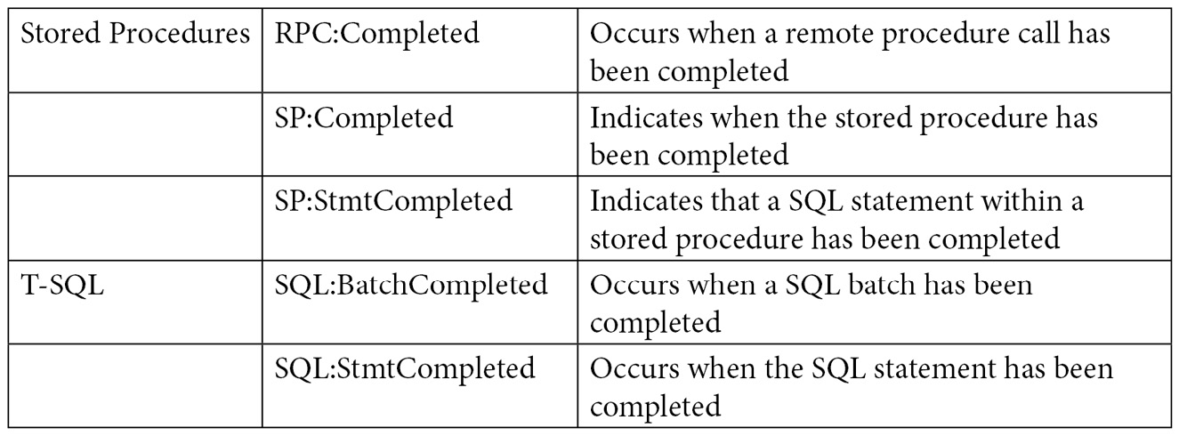
Although you can trace dozens of events using SQL Trace, in this section, we will focus on the ones you can use to measure query resource usage. Because running a trace can take some resources itself, usually, you would only want to run it when you are troubleshooting a query problem, instead of running it all the time. Here are the main trace events we are concerned with regarding query resources usage:

The following screenshot shows an example of such a trace configuration on SQL Server Profiler. Usually, you would want to use Profiler to run the trace for a very short time. If you need to run the trace for, say, hours or a few days, a server trace may be a better choice because it uses fewer resources. The previous chapter showed how you can use Profiler to script and run a server trace:

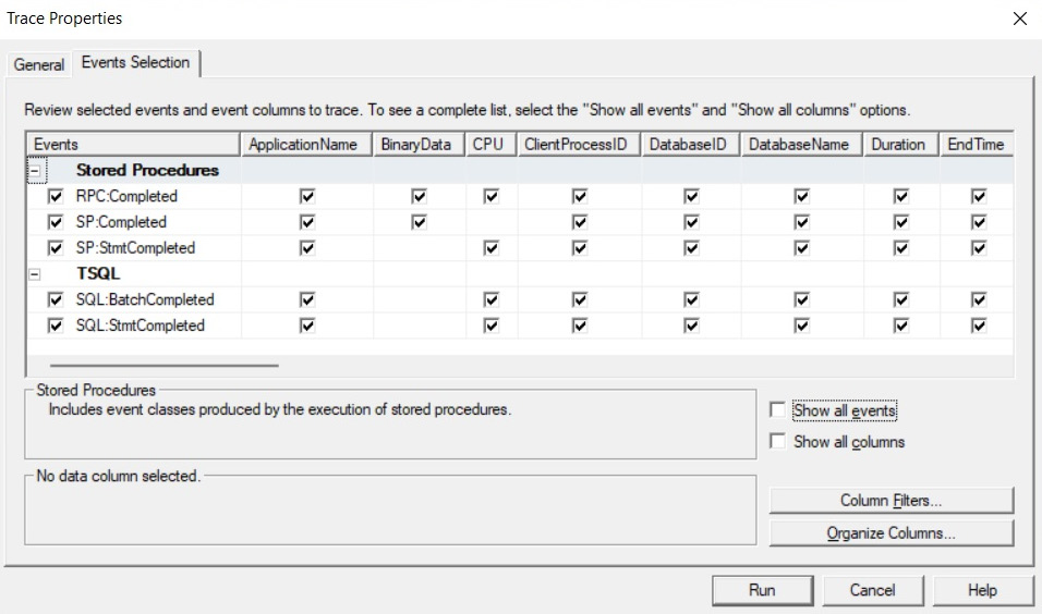
Figure 2.1 – Trace configuration using SQL Server Profiler

Now, let’s see how it works. Run Profiler and select the previous five listed events. Run the trace and then execute the following ad hoc query in Management Studio:

SELECT * FROM Sales.SalesOrderDetail WHERE SalesOrderID = 60677

This query execution will trigger the following events:

SQL:StmtCompleted. SELECT * FROM Sales.SalesOrderDetail WHERE SalesOrderID = 60677
SQL:BatchCompleted. SELECT * FROM Sales.SalesOrderDetail WHERE SalesOrderID = 60677

You could look for ApplicationName under Microsoft SQL Server Management Studio – Query in case you see more events. You may also consider filtering by SPID using Profiler’s filtering capabilities.

Now, let’s say we create and execute the same query as part of a simple stored procedure, like so:

CREATE PROC test
AS
SELECT * FROM HumanResources.Employee WHERE BusinessEntityID = 229

Let’s run it:

EXEC test

Here, we would hit the following events:

SP:StmtCompleted. SELECT * FROM HumanResources.Employee WHERE BusinessEntityID = 229
SP:Completed. SELECT * FROM HumanResources.Employee WHERE BusinessEntityID = 229
SP:Completed. EXEC test
SQL:StmtCompleted. EXEC test
SQL:BatchCompleted. EXEC test

Only the first three events are related to the execution of the stored procedure per se. The last two events are related to the execution of the batch with the EXEC statement.

So, when would we see an RPC:Completed event? For this, we need a remote procedure call (for example, using a .NET application). For this test, we will use the C# code given in the C# Code for RPS Test sidebar. Compile the code and run the created executable file. Because we are calling a stored procedure inside the C# code, we will have the following events:

SP:Completed. SELECT * FROM HumanResources.Employee WHERE BusinessEntityID = 229
SP:StmtCompleted. SELECT * FROM HumanResources.Employee WHERE BusinessEntityID = 229
SP:Completed. exec dbo.test
RPC:Completed. exec dbo.test

Again, you can look for ApplicationName under .Net SqlClient Data Provider in Profiler in case you see additional events:

C# Code for RPC Test

Although looking at .NET code is outside the scope of this book, you can use the following code for the test:

using System;
using System.Data;
using System.Data.SqlClient;
class Test
{
    static void Main()
    {
        SqlConnection cnn = null;
        SqlDataReader reader = null;
        try
            {
            cnn = new SqlConnection("Data Source=(local);
            Initial Catalog=AdventureWorks2019;Integrated
            Security=SSPI");
            SqlCommand cmd = new SqlCommand();
            cmd.Connection = cnn;
            cmd.CommandText = "dbo.test";
            cmd.CommandType = CommandType.StoredProcedure;
            cnn.Open();
            reader = cmd.ExecuteReader();
            while (reader.Read())
            {
                Console.WriteLine(reader[0]);
            }
            return;
        }
        catch (Exception e)
        {
            throw e;
        }
        finally
        {
            if (cnn != null)
            {
                if (cnn.State != ConnectionState.Closed)
                cnn.Close();
            }
        }
    }
}

To compile the C# code, run the following in a command prompt window:

csc test.cs

You don’t need Visual Studio installed, just Microsoft .NET Framework, which is required to install SQL Server, so it will already be available on your system. You may need to find the CSC executable, though, if it is not included on the system’s PATH, although it is usually inside the C:\Windows\Microsoft.NET directory. You may also need to edit the used connection string, which assumes you are connecting to a default instance of SQL Server using Windows authentication.

We briefly introduced extended events in the previous chapter to show you how to capture execution plans. In this section, we’ll gain more information about this feature, which was introduced with SQL Server 2008. There is another important reason for this: as of SQL Server 2012, SQL Trace has been deprecated, making extended events the tool of choice to provide debugging and diagnostic capabilities in SQL Server. Although explaining extended events in full detail is beyond the scope of this book, this section will give you enough background to get started using this feature to troubleshoot your queries.

In this section, you will be introduced to the basic concepts surrounding extended events, including events, predicates, actions, targets, and sessions. Although we mainly use code for the examples in this book, it is worth showing you the new extended events graphical user interface too, which is useful if you are new to this technology and can also help you script the definition of extended events sessions in pretty much the same way we use Profiler to script a server trace. The extended events graphical user interface was introduced in SQL Server 2012.

One of my favorite things to do with SQL Trace – and now with extended events – is to learn how other SQL Server tools work. You can run a trace against your instance and run any one of the tools to capture all the T-SQL statements sent from the tool to the database engine. For example, I recently troubleshooted a problem with Replication Monitor by capturing all the code this tool was sending to SQL Server. Interestingly, the extended events graphical user interface is not an exception, and you can use it to see how the tool itself works. When you start the tool, it loads all the required extended events information. By tracing it, you can see where the information is coming from. You don’t have to worry about this for now as we will cover it next.

Extended events are designed to have a low impact on server performance. They correspond to well-known points in the SQL Server code, so when a specific task is executing, SQL Server will perform a quick check to find out if any sessions have been configured to listen to this event. If no sessions are active, the event will not fire, and the SQL Server task will continue with no overhead. If, on the other hand, there are active sessions that have the event enabled, SQL Server will collect the required data associated with the event. Then, it will validate the predicate, if any, that was defined for the session. If the predicate evaluates to false, the task will continue with minimal overhead. If the predicate evaluates to true, the actions defined in the session will be executed. Finally, all the event data is collected by the defined targets for later analysis.

You can use the following statement to find out the list of events that are available on the current version of SQL Server. You can create an extended events session by selecting one or more of the following events:

SELECT name, description
FROM sys.dm_xe_objects
WHERE object_type = 'event' AND
(capabilities & 1 = 0 OR capabilities IS NULL)
ORDER BY name

Note that 2,408 events are returned with SQL Server 2022 CTP 2.0, including sp_statement_completed, sql_batch_completed, and sql_statement_completed, which we will discuss later.

Each event has a set of columns that you can display by using the sys.dm_xe_object_columns DMV, as shown in the following code:

SELECT o.name, c.name as column_name, c.description
FROM sys.dm_xe_objects o
JOIN sys.dm_xe_object_columns c
ON o.name = c.object_name
WHERE object_type = 'event' AND
c.column_type <> 'readonly' AND
(o.capabilities & 1 = 0 OR o.capabilities IS NULL)
ORDER BY o.name, c.name

An action is a programmatic response to an event and allows you to execute additional code. Although you can use actions to perform operations such as capturing a stack dump or inserting a debugger break into SQL Server, most likely, they will be used to capture global fields that are common to all the events, such as plan_handle and database_name. Actions are also executed synchronously. You can run the following code to find the entire list of available actions:

SELECT name, description
FROM sys.dm_xe_objects
WHERE object_type = 'action' AND
(capabilities & 1 = 0 OR capabilities IS NULL)
ORDER BY name

Predicates are used to limit the data you want to capture, and you can filter against event data columns or any of the global state data returned by the following query:

SELECT name, description
FROM sys.dm_xe_objects
WHERE object_type = 'pred_source' AND
(capabilities & 1 = 0 OR capabilities IS NULL)
ORDER BY name

The query returns 50 values, including database_id, session_id, and query_hash. Predicates are Boolean expressions that evaluate to either true or false, and they also support short-circuiting, in which an entire expression will evaluate to false as soon as any of its predicates evaluates to false.

Finally, you can use targets to specify how you want to collect the data for analysis; for example, you can store event data in a file or keep it in the ring buffer (a ring buffer is a data structure that briefly holds event data in memory in a circular way). These targets are named event_file and ring_buffer, respectively. Targets can consume event data both synchronously and asynchronously, and any target can consume any event. You can list the six available targets by running the following query:

SELECT name, description
FROM sys.dm_xe_objects
WHERE object_type = 'target' AND
(capabilities & 1 = 0 OR capabilities IS NULL)
ORDER BY name

We will cover how to use all these concepts to create event sessions later in this chapter, but first, we will check out how to find the names of events you may be already familiar with when using SQL Trace.

Mapping SQL Trace events to extended events

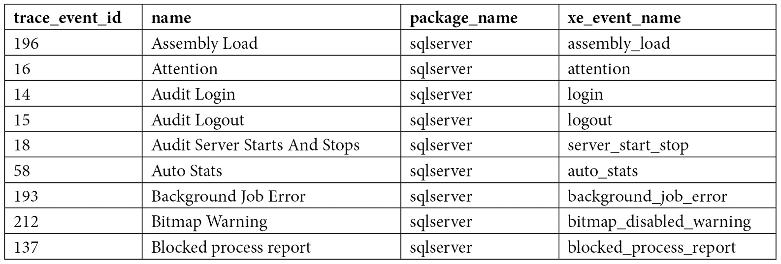
You are probably already familiar with some SQL Trace events or even have trace definitions already configured in your environment. You can use the sys.trace_xe_event_map extended events system table to help you map SQL Trace event classes to extended events. sys.trace_xe_event_map contains one row for each extended event that is mapped to a SQL Trace event class. To see how it works, run the following query:

SELECT te.trace_event_id, name, package_name, xe_event_name
FROM sys.trace_events te
JOIN sys.trace_xe_event_map txe ON te.trace_event_id = txe.trace_event_id
WHERE te.trace_event_id IS NOT NULL
ORDER BY name

The query returns 139 records, some of which are shown here:

In addition, you can use the sys.trace_xe_event_map system table in combination with the sys.fn_trace_geteventinfo function to map the events that have been configured on an existing trace to extended events. The sys.fn_trace_geteventinfo function returns information about a trace currently running and requires its trace ID. To test it, run your trace (explained previously) and run the following statement to get its trace ID. trace_id 1 is usually the default trace. You can easily identify your trace by looking at the path column on the output, where NULL is shown if you are running a Profiler trace:

SELECT * FROM sys.traces

Once you get the trace ID, you can run the following code. In this case, we are using a trace_id value of 2 (used by the sys.fn_trace_geteventinfo function):

SELECT te.trace_event_id, name, package_name, xe_event_name
FROM sys.trace_events te
JOIN sys.trace_xe_event_map txe ON te.trace_event_id = txe.trace_event_id
WHERE te.trace_event_id IN (
SELECT DISTINCT(eventid) FROM sys.fn_trace_geteventinfo(2))
ORDER BY name

If we run the trace we created previously in the SQL Trace section, we will get the following output:

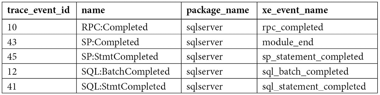
As you can see, the event names of our selected SQL Trace events are very similar to their extended events counterparts, except for SP:Completed, whose extended events name is module_end. Here are the definitions of these events:

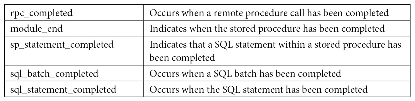
Note

SQL Server comes with several extended events templates. One of them, called Query Detail Sampling, collects detailed statement and error information and includes the five listed events, plus error_reported. It also has some predefined actions and predicates, and it uses the ring_buffer target to collect its data. Its predefined predicated filters only collect 20 percent of the active sessions on the server at any given time, so perhaps that is something you may decide to change.

Working with extended events

At this point, we have enough information to create an extended events session. Extended events include different DDL commands to work with sessions, such as CREATE EVENT SESSION, ALTER EVENT SESSION, and DROP EVENT SESSION. But first, we will learn how to create a session using the extended events graphical user interface, which you can use to easily create and manage extended events sessions, as well as script the generated CREATE EVENT code. To start, in Management Studio, expand the Management and Extended Event nodes and right-click Sessions.

Note

By expanding the Sessions node, you will see three extended events sessions that are defined by default: AlwaysOn_health, telemetry_xevents, and system_health. system_health is started by default every time SQL Server starts, and it is used to collect several predefined events to troubleshoot performance issues. AlwaysOn_health, which is off by default, is a session designed to provide monitoring for Availability Groups, a feature introduced with SQL Server 2012. telemetry_xevents, introduced with SQL Server 2016, is also started by default and includes a large number of events that can also be used to troubleshoot problems with SQL Server. You can see the events, actions, predicates, targets, and configurations that have been defined for these sessions by looking at their properties or scripting them. To script an extended events session in Management Studio, right-click the session and select both Script Session As and CREATE To.

You should see the New Session wizard and the New Session dialog. In this section, we will be briefly introduced to the New Session dialog. Once you select it, you should see the following screen, along with four different pages: General, Events, Data Storage, and Advanced:

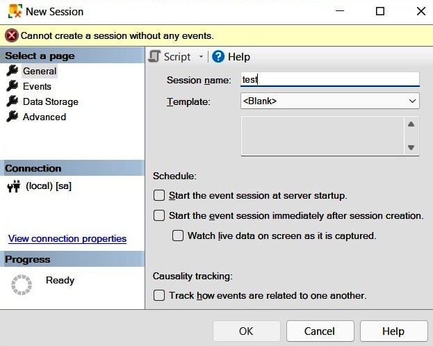
Figure 2.2 – The General page of the New Session dialog

Name the session Test and click the Events page in the selection area on the left.

The Events page allows you to select the events for your session. Because this page may contain a lot of information, you may want to maximize this window. Searching for events in the event library is allowed; for example, because four of the five events we are looking for contain the word completed, you could just type this word to search for them, as shown here:

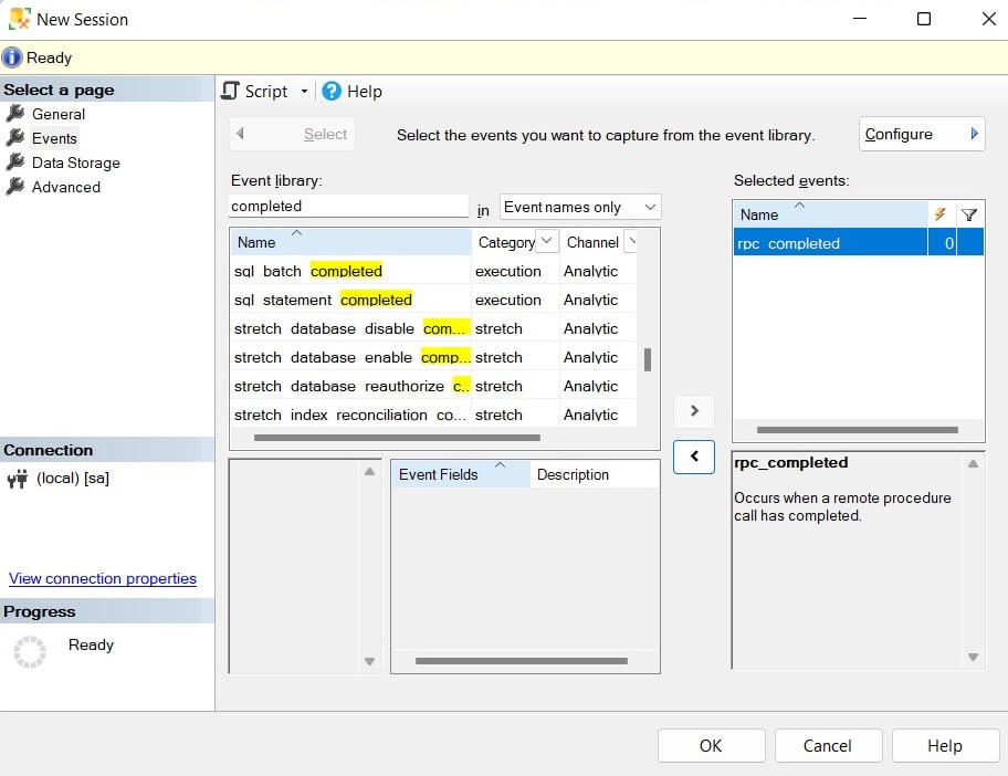
Figure 2.3 – The Events page of the New Session dialog

Click the > button to select the rpc_completed, sp_statement_completed, sql_batch_completed, and sql_statement_completed events. Do a similar search and add the module_end event. The Events page also allows you to define actions and predicates (filters) by clicking the Configure button, which shows the Event Configuration Options section. Click the Configure button, and in addition to selecting our five chosen extended events, check the boxes for the following actions in the Global Fields (Actions) tab: plan_handle, query_hash, query_plan_hash, and sql_text. Your current selection should look as follows:

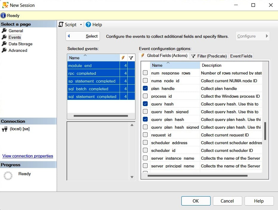
Figure 2.4 – The Event configuration options section of the Events page

Clicking the Data Storage page allows you to select one or more targets to collect your event data. Select the ring_buffer target, as shown in the following screenshot:

Figure 2.5 – The Data Storage page of the New Session dialog

The Advanced page allows you to specify additional options to use with the event session. Let’s keep all the default options as-is on this page.

Finally, as usual in Management Studio, you can also script all the selections you have made by clicking the Script icon at the top of the New Session window. Let’s do just that. This will create the following code, which we can use to create our extended events session:

CREATE EVENT SESSION test ON SERVER
ADD EVENT sqlserver.module_end(
ACTION(sqlserver.plan_handle,sqlserver.query_hash,sqlserver.query_plan_hash,
sqlserver.sql_text)),
ADD EVENT sqlserver.rpc_completed(
ACTION(sqlserver.plan_handle,sqlserver.query_hash,sqlserver.query_plan_hash,
sqlserver.sql_text)),
ADD EVENT sqlserver.sp_statement_completed(
ACTION(sqlserver.plan_handle,sqlserver.query_hash,sqlserver.query_plan_hash,
sqlserver.sql_text)),
ADD EVENT sqlserver.sql_batch_completed(
ACTION(sqlserver.plan_handle,sqlserver.query_hash,sqlserver.query_plan_hash,
sqlserver.sql_text)),
ADD EVENT sqlserver.sql_statement_completed(
ACTION(sqlserver.plan_handle,sqlserver.query_hash,sqlserver.query_plan_hash,
sqlserver.sql_text))
ADD TARGET package0.ring_buffer
WITH (STARTUP_STATE=OFF)

As shown in the previous chapter, we also need to start the extended events session by running the following code:

ALTER EVENT SESSION [test]
ON SERVER
STATE=START

So, at the moment, our session is active, and we just need to wait for the events to occur. To test it, run the following statements:

SELECT * FROM Sales.SalesOrderDetail WHERE SalesOrderID = 60677
GO
SELECT * FROM Person.Address WHERE AddressID = 21
GO
SELECT * FROM HumanResources.Employee WHERE BusinessEntityID = 229
GO

Once you have captured some events, you may want to read and analyze their data. You can use the Watch Live Data feature that was introduced with SQL Server 2012 to view and analyze the extended events data that was captured by the event session, as introduced in the previous chapter. Alternatively, you can use XQuery to read the data from any of the targets. To read the current captured events, run the following code:

SELECT name, target_name, execution_count, CAST(target_data AS xml)
AS target_data
FROM sys.dm_xe_sessions s
JOIN sys.dm_xe_session_targets t
ON s.address = t.event_session_address
WHERE s.name = 'test'

This will produce an output similar to the following:

You can open the link to see the captured data in XML format. Because the XML file would be too large to show in this book, only a small sample of the first event that was captured, showing cpu_time, duration, physical_reads, and logical_reads, and writes, is included here:

<RingBufferTarget truncated="0" processingTime="0" totalEventsProcessed="12"
eventCount="12" droppedCount="0" memoryUsed="5810">
<event name="sql_batch_completed" package="sqlserver"
timestamp="2022-06-01T20:08:42.240Z">
<data name="cpu_time">
<type name="uint64" package="package0" />
<value>0</value>
</data>
<data name="duration">
<type name="uint64" package="package0" />
<value>1731</value>
</data>
<data name="physical_reads">
<type name="uint64" package="package0" />
<value>0</value>
</data>
<data name="logical_reads">
<type name="uint64" package="package0" />
<value>4</value>
</data>
<data name="writes">
<type name="uint64" package="package0" />
<value>0</value>
</data>

However, because reading XML directly is not much fun, we can use XQuery to extract the data from the XML document and get a query like this:

SELECT
event_data.value('(event/@name)[1]', 'varchar(50)') AS event_name,
event_data.value('(event/action[@name="query_hash"]/value)[1]',
'varchar(max)') AS query_hash,
event_data.value('(event/data[@name="cpu_time"]/value)[1]', 'int')
AS cpu_time,
event_data.value('(event/data[@name="duration"]/value)[1]', 'int')
AS duration,
event_data.value('(event/data[@name="logical_reads"]/value)[1]', 'int')
AS logical_reads,
event_data.value('(event/data[@name="physical_reads"]/value)[1]', 'int')
AS physical_reads,
event_data.value('(event/data[@name="writes"]/value)[1]', 'int') AS writes,
event_data.value('(event/data[@name="statement"]/value)[1]', 'varchar(max)')
AS statement
FROM(SELECT evnt.query('.') AS event_data
FROM
(SELECT CAST(target_data AS xml) AS target_data
FROM sys.dm_xe_sessions s
JOIN sys.dm_xe_session_targets t
ON s.address = t.event_session_address
WHERE s.name = 'test'
AND t.target_name = 'ring_buffer'
) AS data
CROSS APPLY target_data.nodes('RingBufferTarget/event') AS xevent(evnt)
) AS xevent(event_data)

This will show an output similar to the following:

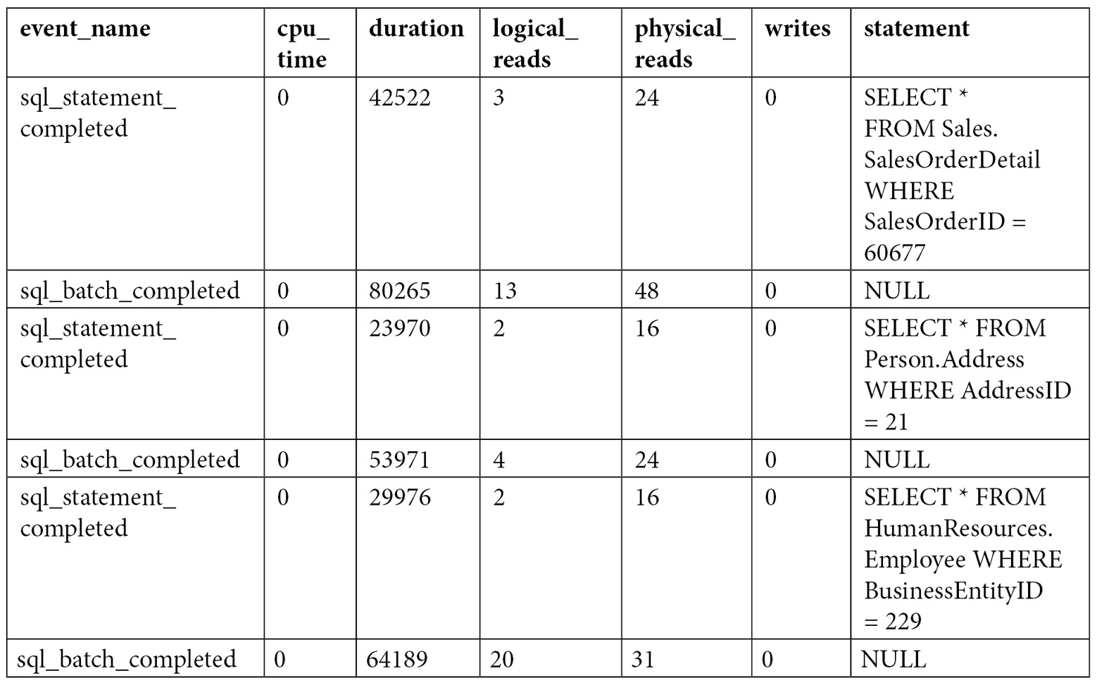
However, using that query, you get all the data for each event, and sometimes, you may want to aggregate the data. For example, sorting the data to look for the greatest CPU consumers may not be enough. As you will also see in other areas of this book, sometimes, a performance problem may be caused by some query that, even if it does not show up on the top 10 consumers, or even the top 100, is executed so many times that its aggregated CPU usage can make it one of the top CPU consumers. You can update the previous query to aggregate this data directly, or you can change it to save the information to a temporary table (for example, using SELECT … INTO) and then group by query_hash and, optionally, sort as needed, as shown here:

SELECT query_hash, SUM(cpu_time) AS cpu_time, SUM(duration) AS duration,
SUM(logical_reads) AS logical_reads, SUM(physical_reads) AS physical_reads,
SUM(writes) AS writes, MAX(statement) AS statement
FROM #eventdata
GROUP BY query_hash

Again, as covered in the previous chapter, after you finish your test, you need to stop and delete the event session. Run the following statements:

ALTER EVENT SESSION [test]
ON SERVER
STATE=STOP
GO
DROP EVENT SESSION [test] ON SERVER

You could also use the file target when collecting large amounts of data or running the session for a long time. The following example is exactly the same as before, but using the file target (note the file definition on the C:\Data folder):

CREATE EVENT SESSION test ON SERVER
ADD EVENT sqlserver.module_end(
ACTION(sqlserver.plan_handle,sqlserver.query_hash,sqlserver.query_plan_hash,
sqlserver.sql_text)),
ADD EVENT sqlserver.rpc_completed(
ACTION(sqlserver.plan_handle,sqlserver.query_hash,sqlserver.query_plan_hash,
sqlserver.sql_text)),
ADD EVENT sqlserver.sp_statement_completed(
ACTION(sqlserver.plan_handle,sqlserver.query_hash,sqlserver.query_plan_hash,
sqlserver.sql_text)),
ADD EVENT sqlserver.sql_batch_completed(
ACTION(sqlserver.plan_handle,sqlserver.query_hash,sqlserver.query_plan_hash,
sqlserver.sql_text)),
ADD EVENT sqlserver.sql_statement_completed(
ACTION(sqlserver.plan_handle,sqlserver.query_hash,sqlserver.query_plan_hash,
sqlserver.sql_text))
ADD TARGET package0.event_file(SET filename=N'C:\Data\test.xel')
WITH (STARTUP_STATE=OFF)

After starting the session and capturing some events, you can query its data by using the following query and the sys.fn_xe_file_target_read_file function:

SELECT
event_data.value('(event/@name)[1]', 'varchar(50)') AS event_name,
event_data.value('(event/action[@name="query_hash"]/value)[1]',
'varchar(max)') AS query_hash,
event_data.value('(event/data[@name="cpu_time"]/value)[1]', 'int')
AS cpu_time,
event_data.value('(event/data[@name="duration"]/value)[1]', 'int')
AS duration,
event_data.value('(event/data[@name="logical_reads"]/value)[1]', 'int')
AS logical_reads,
event_data.value('(event/data[@name="physical_reads"]/value)[1]', 'int')
AS physical_reads,
event_data.value('(event/data[@name="writes"]/value)[1]', 'int') AS writes,
event_data.value('(event/data[@name="statement"]/value)[1]', 'varchar(max)')
AS statement
FROM
(
SELECT CAST(event_data AS xml)
FROM sys.fn_xe_file_target_read_file
(
'C:\Data\test*.xel',
NULL,
NULL,
NULL
)
) AS xevent(event_data)

If you inspect the C:\Data folder, you will find a file with a name similar to test_0_130133932321310000.xel. SQL Server adds "_0_" plus an integer representing the number of milliseconds since January 1, 1600, to the specified filename. You can inspect the contents of a particular file by providing the assigned filename or by using a wildcard (such as the asterisk shown in the preceding code) to inspect all the available files. For more details on using the file target, see the SQL Server documentation. Again, don’t forget to stop and drop your session when you finish testing.

Finally, we will use extended events to show you how to obtain the waits for a specific query, something that was not even possible before extended events. You must use the wait_info event and select any of the many available fields (such as username or query_hash) or selected actions to apply a filter (or predicate) to it. In this example, we will use session_id. Make sure to replace session_id as required if you are testing this code:

CREATE EVENT SESSION [test] ON SERVER
ADD EVENT sqlos.wait_info(
WHERE ([sqlserver].[session_id]=(61)))
ADD TARGET package0.ring_buffer
WITH (STARTUP_STATE=OFF)

Start the event:

ALTER EVENT SESSION [test]
ON SERVER
STATE=START

Run some transactions but note that they need to be executed in the session ID you specified (and they need to create waits). For example, run the following query:

SELECT * FROM Production.Product p1 CROSS JOIN
Production.Product p2

Then, you can read the captured data:

SELECT
event_data.value('(event/@name)[1]', 'varchar(50)') AS event_name,
event_data.value('(event/data[@name="wait_type"]/text)[1]', 'varchar(40)')
AS wait_type,
event_data.value('(event/data[@name="duration"]/value)[1]', 'int')
AS duration,
event_data.value('(event/data[@name="opcode"]/text)[1]', 'varchar(40)')
AS opcode,
event_data.value('(event/data[@name="signal_duration"]/value)[1]', 'int')
AS signal_duration
FROM(SELECT evnt.query('.') AS event_data
FROM
(SELECT CAST(target_data AS xml) AS target_data
FROM sys.dm_xe_sessions s
JOIN sys.dm_xe_session_targets t
ON s.address = t.event_session_address
WHERE s.name = 'test'
AND t.target_name = 'ring_buffer'
) AS data
CROSS APPLY target_data.nodes('RingBufferTarget/event') AS xevent(evnt)
) AS xevent(event_data)

Here is the output on my system:

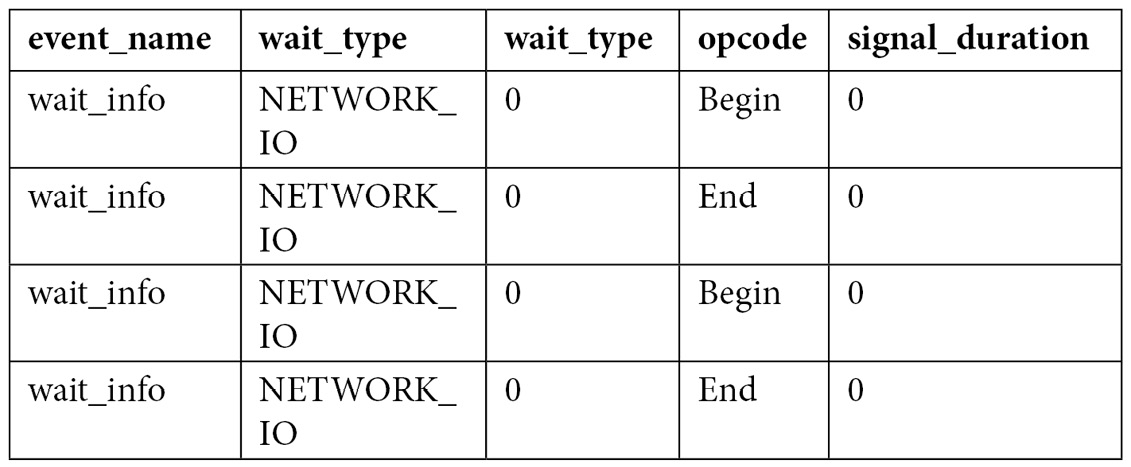
Again, this is another example where aggregating the captured data would be beneficial. Finally, don’t forget to stop and drop your event session, as indicated previously.

So, now that we have covered several features that we can use to collect query performance information, such as DMVs, DMFs, SQL Trace, and extended events, let’s close this chapter with the Data Collector. The Data Collector is a tool that’s designed to collect performance data and is especially useful in cases where you do not have access to a dedicated third-party tool.

There may be cases when a performance problem occurs and there is little or no information available to troubleshoot it. For example, you may receive a notification that CPU percentage usage was 100 percent for a few minutes, thus slowing down your application, but by the time you connected to the system to troubleshoot, the problem is already gone. Many times, a specific problem is difficult to reproduce, and the only choice is to enable a trace or some other collection of data and wait until the problem happens again.

This is where proactively collecting performance data is extremely important, and the Data Collector, a feature introduced with SQL Server 2008, can help you to do just that. The Data Collector allows you to collect performance data, which you can use immediately after a performance problem occurs. You only need to know the time the problem occurred and start looking at the collected data around that period.

Explaining the Data Collector would take an entire chapter, if not an entire book. Therefore, this section aims to show you how to get started. You can find more details about the Data Collector by reading the SQL Server documentation or by reading the Microsoft white paper Using Management Data Warehouse for Performance Monitoring by Ken Lassesen.

Configuration

The Data Collector is not enabled by default after you install SQL Server. To configure it, you need to follow a two-step process:

1. To configure the first part, expand the Management folder in Management Studio, right-click the Data Collection node, and select Tasks, followed by Configure Management Data Warehouse. This will run the Configure Management Data Warehouse Wizard. Click Next on the Welcome screen. This will take you to the Configure Management Data Warehouse Storage screen, as shown in the following screenshot. This screen allows you to select the database you will use to collect data. Optionally, you can create a new database by selecting the New button:

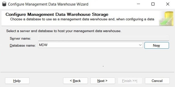
Figure 2.6 – The Configure Management Data Warehouse Storage screen

2. Select an existing database, or create a new one, and then click Next. The following screen, Map Logins and Users, as shown in the following screenshot, allows you to map logins and users to management data warehouse roles:

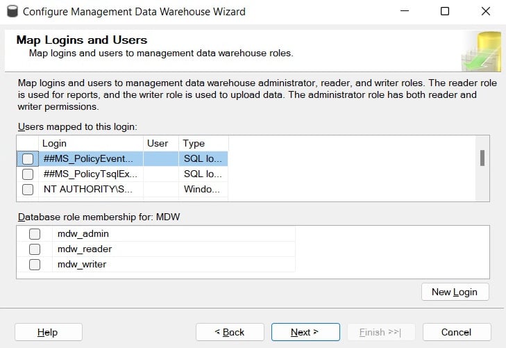
Figure 2.7 – The Map Logins and Users screen

3. Click Next. The Complete the Wizard screen will appear.
4. On the Complete the Wizard screen, click Finish. You will see the Configure Data Collection Wizard Progress screen. Make sure all the steps shown are executed successfully and click the Close button. This step configures the management data warehouse database, and, among other objects, it will create a collection of tables, some of which we will query directly later in this section.
5. To configure the second step, right-click Data Collection again and select Tasks, followed by Configure Data Collection. This will open the Configure Data Collection Wizard screen. Click Next. You should see Setup Data Collection Sets, as shown in the following screenshot:

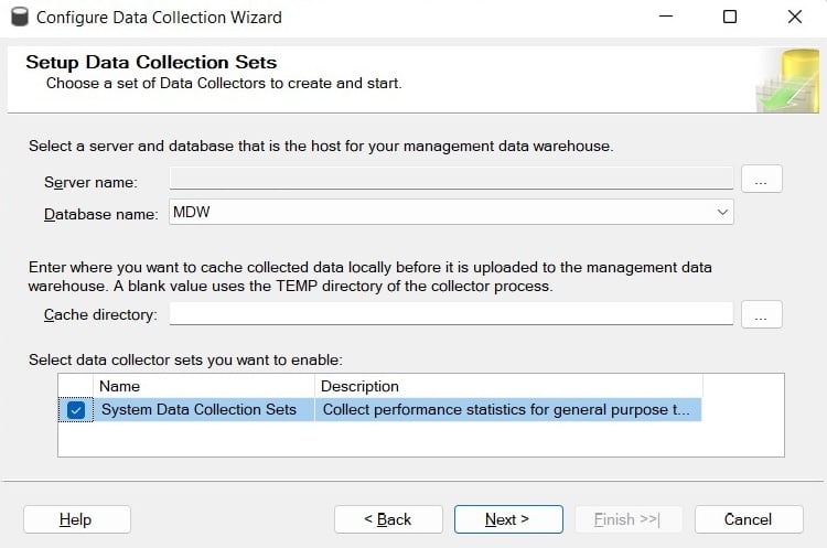
Figure 2.8 – The Setup Data Collection Sets screen

This is where you select the database to be used as the management data warehouse, which is the database you configured in Step 1. You can also configure the cache directory, which is used to collect the data before it is uploaded to the management data warehouse.

6. Finally, you need to select the Data Collector sets that you want to enable, which in our case requires selecting System Data Collection Sets. Although it is the only data collector set available on SQL Server 2022, some others have been available on previous versions, such as the Transaction Performance Collection Set, which was used by the In-Memory OLTP feature. Click Next and then Finish on the Complete the Wizard screen.

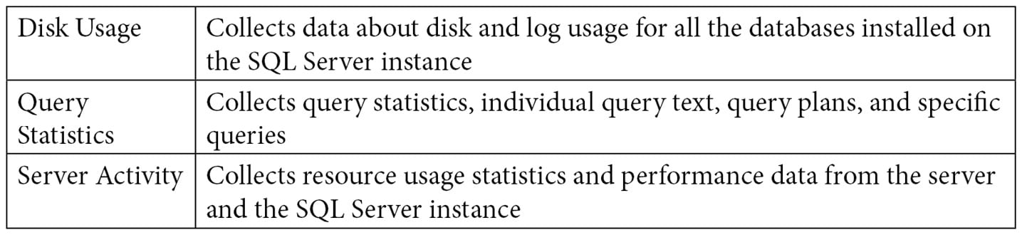
Once you’ve configured the Data Collector, among other items, you will see the three enabled system data collection sets: Disk Usage, Query Statistics, and Server Activity. The Utility Information collection set is disabled by default, and it will not be covered in this book. The following data was collected by the System Data Collection Sets:

In addition, it is strongly recommended that you install the optional Query Hash Statistics collection set, which you can download from http://blogs.msdn.com/b/bartd/archive/2010/11/03/query-hash-statistics-a-query-cost-analysis-tool-now-available-for-download.aspx. The Query Hash Statistics collection set, which unfortunately is not included as part of SQL Server 2022, is based on the query_hash and plan_hash values, as explained earlier in this chapter. It collects historical query and query plan fingerprint statistics, allowing you to easily see the true cumulative cost of the queries in each of your databases. After you install the Query Hash Statistics collection set, you will need to disable the Query Statistics collection set because it collects the same information.

7. Finally, you need to be aware of the following SQL Server Agent jobs that were created:
   • collection_set_1_noncached_collect_and_upload
   • collection_set_2_collection
   • collection_set_2_upload
   • collection_set_3_collection
   • collection_set_3_upload
   • mdw_purge_data_[MDW]
   • syspolicy_purge_history

Using the Data Collector

The next thing you want to do is become familiar with the Data Collector – mostly, the reports available and the information that’s collected on each table. To start looking at the reports, right-click Data Collection and select Reports, Management Data Warehouse, and Server Activity History. Assuming enough data has already been collected, you should see a report similar to the one shown in the following screenshot (only partly shown):

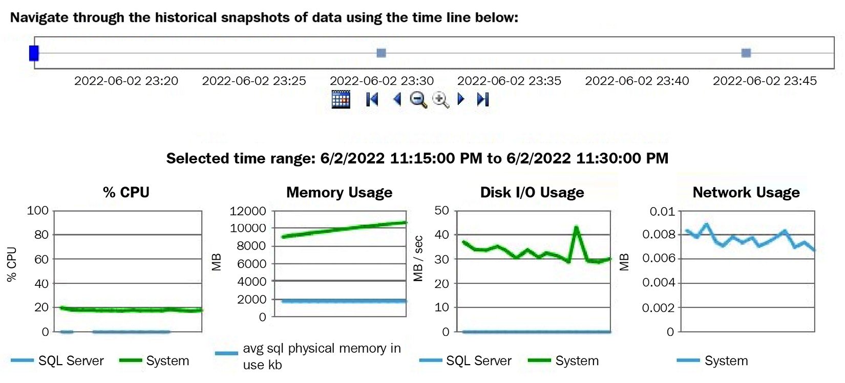
Figure 2.9 – The Server Activity History report

Clicking the SQL Server section of the % CPU graph will take you to the Query Statistics History report. You can also reach this report by right-clicking Data Collection and then selecting Reports, Management Data Warehouse, and Query Statistics History. In both cases, you will end up with the report shown in the following screenshot (only partly shown):

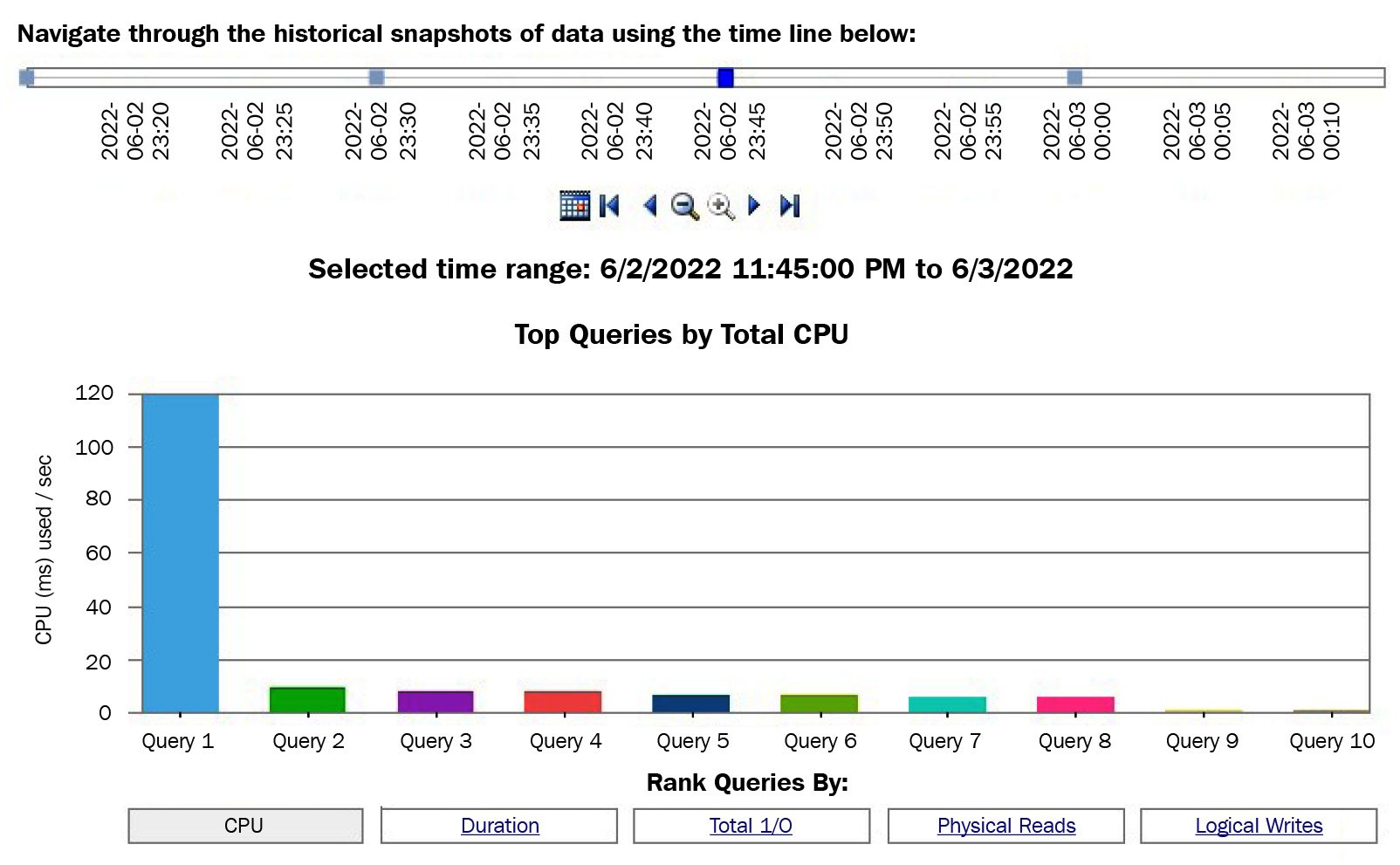
Figure 2.10 – The Query Statistics History report

Running the Query Statistics History report will show you the top 10 most expensive queries ranked by CPU usage, though you also have the choice of selecting the most expensive queries by duration, total I/O, physical reads, and logical writes. The Data Collector includes other reports, and as you’ve seen already, some reports include links to navigate to other reports for more detailed information.

Querying the Data Collector tables

More advanced users will want to query the Data Collector tables directly to create reports or look deeper into the collected data. Creating custom collection sets is also possible and may be required when you need to capture data that the default installation is not collecting. Having custom collection sets would, again, require you to create your own queries and reports.

For example, the Data Collector collects multiple performance counters, which you can see by looking at the properties of the Server Activity collection set. To do this, expand both the Data Collection and System Data Collection sets, right-click the Server Activity collection set, and select Properties. In the Data Collection Set Properties window, select Server Activity – Performance Counters in the Collection Items list box and look at the Input Parameters window. Here is a small sample of these performance counters:

\Memory \% Committed Bytes In Use
\Memory \Available Bytes
\Memory \Cache Bytes
\Memory \Cache Faults/sec
\Memory \Committed Bytes
\Memory \Free & Zero Page List Bytes
\Memory \Modified Page List Bytes
\Memory \Pages/sec
\Memory \Page Reads/sec
\Memory \Page Write/sec
\Memory \Page Faults/sec
\Memory \Pool Nonpaged Bytes
\Memory \Pool Paged Bytes

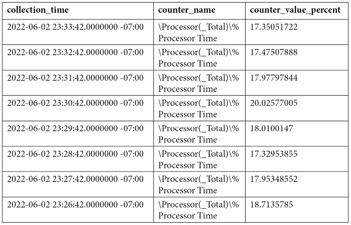
You can also see a very detailed definition of the performance counters that have been collected in your instance by looking at the snapshots.performance_counter_instances table. Performance counters’ data is then stored in the snapshots.performance_counter_values table. One of the most used performance counters by database administrators is '\Processor(_Total)\% Processor Time', which allows you to collect the processor percentage usage. We can use the following query to get the collected data:

SELECT sii.instance_name, collection_time, [path] AS counter_name,
formatted_value AS counter_value_percent
FROM snapshots.performance_counter_values pcv
JOIN snapshots.performance_counter_instances pci
ON pcv.performance_counter_instance_id = pci.performance_counter_id
JOIN core.snapshots_internal si ON pcv.snapshot_id = si.snapshot_id
JOIN core.source_info_internal sii ON sii.source_id = si.source_id
WHERE pci.[path] = '\Processor(_Total)\% Processor Time'
ORDER BY pcv.collection_time desc

An output similar to the following will be shown:

There are some other interesting tables, at least from the point of view of query data collection, you may need to query directly. The Query Statistics collection set uses queries defined in the QueryActivityCollect.dtsx and QueryActivityUpload.dtsx SSIS packages, and the collected data is loaded into the snapshots.query_stats, snapshots.notable_query_text, and snapshots.notable_query_plan tables. These tables collect query statistics, query text, and query plans, respectively. If you installed the Query Hash Statistics collection set, the QueryHashStatsPlanCollect and QueryHashStatsPlanUpload packages will be used instead. Another interesting table is snapshots.active_sessions_and_requests, which collects information about SQL Server sessions and requests.

This chapter has provided you with several tuning techniques you can use to find out how your queries are using system resources such as disk and CPU. First, we explained some essential DMVs and DMFs that are very useful for tracking expensive queries. Two features that were introduced with SQL Server 2008, extended events and the Data Collector, were explained as well, along with how they can help capture events and performance data. We also discussed SQL Trace, a feature that has been around in all the SQL Server versions as far as any of us can remember.

So, now that we know how to find the expensive queries in SQL Server, what’s next? Our final purpose is to do something to improve the performance of the query. To achieve that, we will cover different approaches in the coming chapters. Is just a better index needed? Maybe your query is sensitive to different parameters, or maybe the query optimizer is not giving you a good execution plan because a used feature does not have good support for statistics. We will cover these and many other issues in the following chapters.

Once we have found the query that may be causing the problem, we still need to troubleshoot what the problem is and find a solution to it. Many times, we can troubleshoot what the problem is just by inspecting all the rich information that’s available in the query execution plan. To do that, we need to dive deeper into how the query optimizer works and what the different operators the execution engine provides. We will cover those topics in detail in the following two chapters.