Machine learning teaches machines to learn to carry out tasks by themselves. It is that simple. The complexity comes with the details, and that is most likely the reason you are reading this book.

Maybe you have too much data and too little insight. Maybe you hope that, by using machine learning algorithms, you can solve this challenge, so you started digging into the algorithms. But perhaps after a while you became puzzled: which of the myriad of algorithms should you actually choose?

Alternatively, maybe you are simply more generally interested in machine learning and you have been reading blogs and articles about it for some time. Everything seemed to be magic and cool, so you started your exploration and fed some data into a decision tree or a support vector machine. However, after you successfully applied these to some other data, perhaps you wondered: was the whole setting right? Did you get optimal results? How do you know that there are no better algorithms? Or whether your data was the right kind?

Welcome to the club! All of us authors were once at those stages, looking for information that tells the stories behind the theoretical textbooks about machine learning. It turned out that much of that information was black art, not usually taught in standard text books. So, in a sense, we wrote this book to our younger selves. A book that not only gives a quick introduction to machine learning, but also teaches the lessons we learned during our careers in the field. We hope that it will also give you a smoother entry into one of the most exciting fields in computer science.

The goal of machine learning is to teach machines (software) to carry out tasks by providing them with a couple of examples (that is, examples of how to do or not do the task). Let's assume that each morning when you turn on your computer, you perform the same task of moving emails around so that only emails belonging to the same topic end up in the same folder. After some time, you might feel bored and think of automating this chore. One way would be to start analyzing your brain and write down all the rules and decisions that your brain processes while you are shuffling your emails. However, this will be quite cumbersome and always imperfect. While you will miss some rules, you will overspecify others. A better and more future-proof way of doing this would be to automate this process by choosing a set of email meta information and body/folder name pairs and letting an algorithm come up with the best rule set. The pairs would be your training data, and the resulting rule set (also called a model) could then be applied to future emails that you have not yet seen. This is machine learning in its simplest form.

Of course, machine learning is not a brand new field in itself. Quite the contrary: its success in recent years can be attributed to the pragmatic way that it uses rock-solid techniques and insights from other successful fields, such as statistics. In these fields, the purpose is for us humans to get insights into the data—for example, by learning more about the underlying patterns and relationships within it. As you read more and more about successful applications of machine learning (you have checked out www.kaggle.com already, haven't you?), you will see that applied statistics is a common field among machine learning experts.

As you will see later, the process of coming up with a decent machine learning approach is never easy. Instead, you will find yourself going back and forth in your analysis, trying out different versions of your input data on diverse sets of machine learning algorithms. It is this exploratory nature that lends itself perfectly to Python. Being an interpreted, high-level programming language, it seems that Python has been designed exactly for this process of trying out different things. What is more, it even does this fast. Sure, it is slower than C or many other natively compiled programming languages. Nevertheless, with the myriad of easy-to-use libraries that are often written in C, you don't have to sacrifice speed for agility.

This book will give you a broad overview of what types of learning algorithms are currently most used in the diverse fields of machine learning, and what to watch out for when applying them. From our own experience, however, we know that doing the cool stuff—that is, using and tweaking machine learning algorithms, such as support vector machines, nearest neighbor searches, or ensembles thereof—will only consume a tiny fraction of the overall time that a good machine learning expert will spend doing the same thing. Looking at the following typical workflow, we can see that most of the time will be spent on rather mundane tasks:

• Reading the data and cleaning it
• Exploring and understanding the input data
• Analyzing how to best present the data to the learning algorithm
• Choosing the right model and learning algorithm
• Measuring the performance correctly

When talking about exploring and understanding the input data, we will need to use a bit of statistics and basic math. However, while doing this, you will see that those topics that seemed so dry in your math class can actually be really exciting when you use them to look at interesting data.

The journey starts when you read in the data. When you have to answer questions such as, "How do I handle invalid or missing values?", you will see that this is more an art than a precise science, and a very rewarding art, as doing this part correctly will open your data to more machine learning algorithms and hence increase the likelihood of success.

With the data ready and waiting in your program's data structures, you will want to get a real feeling for what animal you are working with. Do you have enough data to answer your questions? If not, you might want to think about additional ways to get more of it. Perhaps you even have too much data. In that case, you probably want to think about how to best extract a sample of it.

Often, you will not feed the data directly into your machine learning algorithm. Instead, you will find that you can refine parts of the data before training. Oftentimes, the machine learning algorithm will reward you with increased performance. You will even find that a simple algorithm with refined data generally outperforms a very sophisticated algorithm with raw data. This part of the machine learning workflow is called feature engineering, and, most of the time, it is a very exciting and rewarding challenge. You will immediately see the results of your previous creative and intelligent efforts.

Choosing the right learning algorithm, then, is not simply a shoot-out of the three or four that are in your toolbox (there will be more; you will see). It is more a thoughtful process of weighing different performance and functional requirements. Do you need a fast result and are willing to sacrifice quality? Or would you rather spend more time to get the best possible result? Do you have a clear idea of future data, or should you be a bit more conservative on that side?

Finally, measuring performance is the part of the process that has the most potential pitfalls for the aspiring machine learner. There are easy mistakes to avoid, such as testing your approach with the same data on which you have trained. But there are more difficult ones as well, such as using imbalanced training data. Again, the data is the part that determines whether your undertaking will fail or succeed.

We see that only the fourth point deals with the fancy algorithms. Nevertheless, we hope that this book will convince you that the other four tasks are not simply chores, but can be equally exciting. Our hope is that, by the end of the book, you will have truly fallen in love with data instead of learning algorithms.

To that end, we will not overwhelm you with the theoretical aspects of the diverse machine learning algorithms, as there are already excellent books in that area (you will find pointers in the appendix). Instead, we will try to provide you with an understanding of the underlying approaches in the individual chapters—just enough for you to get an idea and be able to undertake your first steps. Hence, this book is by no means the definitive guide to machine learning—it is more of a starter kit. We hope that it ignites your curiosity enough to keep you eager in trying to learn more and more about this interesting field.

In the rest of this chapter, we will set up and get to know the basic Python libraries of NumPy and SciPy, and then train our first machine learning algorithm using scikit-learn. During this, we will introduce basic machine learning concepts that will be used throughout the book. The rest of the chapters will then go into more detail about the five steps described earlier, highlighting different aspects of machine learning in Python using diverse application scenarios.

While we have tried to provide all the code required to convey the book's ideas, we don't want to bore you with repetitive code snippets. Instead, we have created self-contained Jupyter notebooks (http://jupyter.org) that you can find via Git from https://github.com/PacktPublishing/Building-Machine-Learning-Systems-with-Python-Third-edition.

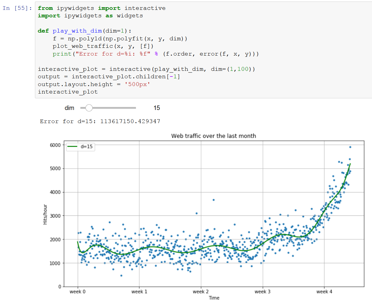
If you don't have Jupyter already, simply install it with pip install jupyter and then run it with jupyter notebook. It provides a much richer experience; for example, it directly integrates charts into it. Once you have cloned the Git repository of the book's code, you can simply follow along by hitting Shift + Enter. As a bonus, you will find that it has interactive widgets that let you play with the code:

We have tried to convey every idea necessary to reproduce the steps throughout this book. Nevertheless, there will be situations where you are stuck. The reasons might range from simple typos over odd combinations of package versions to problems in understanding.

There are many different ways to get help. Most likely, your problem will already have been raised and solved in the following excellent Q&A sites:

• http://stats.stackexchange.com: This Q&A site is named Cross Validated, similar to MetaOptimize, but is focused more on statistical problems.
• http://stackoverflow.com: This Q&A site is much like the previous one, but with a broader focus on general programming topics. It contains, for example, more questions on some of the packages that we will use in this book, such as SciPy or Matplotlib.
• https://freenode.net/: This is the IRC channel focused on machine learning topics. It is a small but very active and helpful community of machine learning experts.

As stated at the beginning, this book is intended to help you get started quickly on your machine learning journey. Therefore, we highly encourage you to build up your own list of machine learning-related blogs and check them out regularly. This is the best way to get to know what works and what doesn't.

The only blog we want to highlight right here (though there there are more in the appendix) is http://blog.kaggle.com, the blog of the company, Kaggle, which hosts machine learning competitions. Typically, they encourage the winners of the competitions to write down how they approached the competition, what strategies did not work, and how they arrived at the winning strategy. Even if you don't read anything else, this is a must.

Assuming that you have Python already installed (anything at least as recent as 3 should be fine), we need to install NumPy and SciPy for numerical operations, as well as Matplotlib for visualization.

Before we can talk about concrete machine learning algorithms, we have to talk about how best to store the data we will chew through. This is important as the most advanced learning algorithm will not be of any help to us if it will never finish. This may be simply because the mere process of accessing the data is too slow, or maybe its representation forces the operating system to swap all day. Add to this the fact that Python is an interpreted language (a highly optimized one, though) that is slow for many numerically heavy algorithms compared to C or Fortran. So we might ask why on earth so many scientists and companies are betting their fortune on Python even in highly computation-intensive areas.

The answer is that, in Python, it is very easy to offload number crunching tasks to the lower layer in the form of C or Fortran extensions, and that is exactly what NumPy and SciPy do (see https://scipy.org). NumPy provides the support of highly optimized multidimensional arrays, which are the basic data structure of most state-of-the-art algorithms. SciPy uses those arrays to provide a set of fast numerical recipes. Matplotlib (http://matplotlib.org) is probably the most convenient and feature-rich library to plot high-quality graphs using Python. Finally, TensorFlow is one of the leading neural network packages for Python (we will explain what this package is about in a subsequent chapter).

Luckily, for all major operating systems—that is, Windows, Mac, and Linux—there are targeted installers for NumPy, SciPy, Matplotlib, and TensorFlow. If you are unsure about the installation process, you might want to install the Anaconda Python distribution (which you can access at https://www.anaconda.com/download), which is maintained and developed by Travis Oliphant, a founding contributor of SciPy. Luckily, Anaconda is already fully compatible with Python 3—the Python version we will be using throughout this book.

Let's walk quickly through some basic NumPy examples and then take a look at what SciPy provides on top of it. On the way, we will get our feet wet with plotting using the marvelous matplotlib package.

For an in-depth explanation, you might want to take a look at some of the more interesting examples of what NumPy has to offer at https://docs.scipy.org/doc/numpy/user/quickstart.html.

You will also find the NumPy Beginner's Guide - Second Edition by Ivan Idris, from Packt Publishing, very valuable. Additional tutorial style guides can be found at http://www.scipy-lectures.org, and the official SciPy tutorial can be found at http://docs.scipy.org/doc/scipy/reference/tutorial.

So, let's import NumPy and play with it a bit. For that, we need to start the Python interactive shell:

>>> import numpy
>>> numpy.version.full_version 
1.13.3

As we do not want to pollute our namespace, we certainly should not use the following code:

>>> from numpy import *

If we do this, then, for instance, numpy.array will potentially shadow the array package that is included in standard Python. Instead, we will use the following convenient shortcut:

>>> import numpy as np
>>> a = np.array([0,1,2,3,4,5])
>>> a
array([0, 1, 2, 3, 4, 5])
>>> a.ndim 
1
>>> a.shape 
(6,)

With the previous code snippet, we created an array in the same way that we would create a list in Python. However, the NumPy arrays have additional information about the shape. In this case, it is a one-dimensional array of six elements. That's no surprise so far.

We can now transform this array into a two-dimensional matrix:

>>> b = a.reshape((3,2))
>>> b
array([[0, 1],
       [2, 3],
       [4, 5]])
>>> b.ndim 
2
>>> b.shape
(3, 2)

It is important to realize just how much the NumPy package is optimized. For example, doing the following avoids copies wherever possible:

>>> b[1][0] = 77
>>> b
array([[ 0, 1],
       [77, 3],
       [ 4, 5]])
>>> a
array([ 0, 1, 77, 3, 4, 5])

In this case, we have modified the value 2 to 77 in b, and we immediately see the same change reflected in a, as well. Keep in mind that whenever you need a true copy, you can always perform the following:

>>> c = a.reshape((3,2)).copy()
>>> c
array([[ 0, 1],
       [77, 3],
       [ 4, 5]])
>>> c[0][0] = -99
>>> a
array([ 0, 1, 77, 3, 4, 5])
>>> c
array([[-99, 1],
       [ 77, 3],
       [ 4, 5]])

Note that, here, c and a are totally independent copies.

Another big advantage of NumPy arrays is that the operations are propagated to the individual elements. For example, multiplying a NumPy array will result in an array of the same size (including all of its elements) being multiplied:

>>> d = np.array([1,2,3,4,5])
>>> d*2
array([ 2, 4, 6, 8, 10])

This is also true for other operations:

>>> d**2
array([ 1, 4, 9, 16, 25])

Contrast that with ordinary Python lists:

>>> [1,2,3,4,5]*2
[1, 2, 3, 4, 5, 1, 2, 3, 4, 5]
>>> [1,2,3,4,5]**2
Traceback (most recent call last): 
  File "<stdin>", line 1, in <module>
TypeError: unsupported operand type(s) for ** or pow(): 'list' and 'int'

Of course, by using NumPy arrays, we sacrifice the agility Python lists offer. Simple operations, such as adding or removing elements, are a bit complex for NumPy arrays. Luckily, we have both at our hands, and we will use the right one for the task at hand.

Part of the power of NumPy comes from the versatile ways in which its arrays can be accessed.

In addition to normal list indexing, it allows you to use arrays themselves as indices by performing the following:

>>> a[np.array([2,3,4])] 
array([77, 3, 4])

Coupled with the fact that conditions are also propagated to individual elements, we gain a very convenient way to access our data, using the following:

>>> a>4
array([False, False, True, False, False, True], dtype=bool)
>>> a[a>4]
array([77, 5])

By performing the following command, we can trim outliers:

>>> a[a>4] = 4
>>> a
array([0, 1, 4, 3, 4, 4])

As this is a frequent use case, there is a special clip function for it, clipping the values at both ends of an interval with one function call:

>>> a.clip(0,4)
array([0, 1, 4, 3, 4, 4])

The power of NumPy's indexing capabilities comes in handy when preprocessing data that we have just read in from a text file. Most likely, this will contain invalid values that we will mark as not being real numbers, using numpy.NAN, as shown in the following code:

>>> # let's pretend we have read this from a text file:
>>> c = np.array([1, 2, np.NAN, 3, 4])
array([ 1., 2., nan, 3., 4.])
>>> np.isnan(c)
array([False, False, True, False, False], dtype=bool)
>>> c[~np.isnan(c)]
array([ 1., 2., 3., 4.])
>>> np.mean(c[~np.isnan(c)]) 
2.5

Let's compare the runtime behavior of NumPy to normal Python lists. In the following code, we will calculate the sum of all squared numbers from 1 to 1,000 and see how much time it will take. We will perform it 10,000 times and report the total time so that our measurement is accurate enough:

import timeit

normal_py_sec = timeit.timeit('sum(x*x for x in range(1000))',
                              number=10000)
naive_np_sec = timeit.timeit('sum(na*na)',
                             setup="import numpy as np; na=np.arange(1000)", 
                             number=10000)
good_np_sec = timeit.timeit('na.dot(na)',
                            setup="import numpy as np; na=np.arange(1000)", 
                            number=10000)

print("Normal Python: %f sec" % normal_py_sec) 
print("Naive NumPy: %f sec" % naive_np_sec) 
print("Good NumPy: %f sec" % good_np_sec) 

Executing this will output

Normal Python: 1.571072 sec
Naive NumPy: 1.621358 sec 
Good NumPy: 0.035686 sec

We can make two interesting observations from this code. Firstly, just using NumPy as data storage (naive NumPy) takes longer, which is surprising since it seems it should be much faster, as it is written as a C extension. One reason for this increased processing time is that the access of individual elements from Python itself is rather costly. Only when we are able to apply algorithms inside the optimized extension code do we get speed improvements. The other observation is quite a tremendous one: using the dot() function of NumPy, which does exactly the same, allows us to be more than 44 times faster. In summary, in every algorithm we are about to implement, we should always look at how we can move loops over individual elements from Python to some of the highly optimized NumPy or SciPy extension functions.

However, this speed comes at a price. Using NumPy arrays, we no longer have the incredible flexibility of Python lists, which can hold basically anything. NumPy arrays always have only one data type:

>>> a = np.array([1,2,3])
>>> a.dtype 
dtype('int32')

If we try to use elements of different types, such as the ones shown in the following code, NumPy will do its best to correct them to be the most reasonable common data type:

>>> np.array([1, "stringy"]) 
array(['1', 'stringy'], dtype='<U11')
>>> np.array([1, "stringy", {1, 2, 3}])
array([1, 'stringy', {1, 2, 3}], dtype=object)

On top of the efficient data structures of NumPy, SciPy offers a magnitude of algorithms for working on those arrays. Whatever numerical heavy algorithm you take from current books on numerical recipes, you will most likely find support for them in SciPy in one way or another. Whether it is matrix manipulation, linear algebra, optimization, clustering, spatial operations, or even fast Fourier transformation, the toolbox is readily filled. Therefore, it is a good habit to always inspect the scipy module before you start implementing a numerical algorithm.

For convenience, the complete namespace of NumPy is also accessible via SciPy. So, from now on, we will use NumPy's machinery via the SciPy namespace. You can check this by easily comparing the function references of any base function, such as the following:

>>> import scipy, numpy
>>> scipy.version.full_version 
1.0.0
>>> scipy.dot is numpy.dot 
True

The diverse algorithms are grouped into the following toolboxes:

The toolboxes that are most pertinent to our goals are scipy.stats, scipy.interpolate, scipy.cluster, and scipy.signal. For the sake of brevity, we will briefly explore some features of the stats package and explain the others when they show up in the individual chapters.

In machine learning, what we are doing is asking a question and answering it. From the samples we have, we create a question that is the learning aspect of the model. Answering the question involves using the model for new samples.

If the workflow involves preprocessing the features, followed by model training, and finally model usage, then the preprocessing features step can be linked to the assumptions that we make when asking a question. For instance, the question can be, "Are these images of cats, knowing that cats have two ears, two eyes, a nose, a mouth, and whiskers?"

Our assumptions here are linked to how the images will be preprocessed to get the number of ears, eyes, noses, mouths, and whiskers. This data will be fed into the model during training so that we get answers.

Once the model is trained, we use the same features to get our answer. Of course, with the question we asked earlier, if we feed in images of cats, we will get a positive answer. But if we feed in an image of a tiger, a lion, or a dog, we will also get a positive identification. So the question we asked is not, "Are these images of cats?", but really, "Are these images of cats, knowing that cats have two ears, two eyes, a nose, a mouth, and whiskers?". Our definition of a cat was wrong and lead us to wrong answers.

This is where know-how and practice are important. Designing the right model to answer the question you have been asked is something that anyone can do once this important point has been understood.

Let's get our hands dirty and take a look at our hypothetical web start-up, MLaaS, which sells the service of providing machine learning algorithms via HTTP. With the increasing success of our company, the demand for better infrastructure also increases so that we can serve all incoming web requests successfully. We don't want to allocate too many resources as that would be too costly. On the other hand, we will lose money if we have not reserved enough resources to serve all incoming requests. Now, the question is, when will we hit the limit of our current infrastructure, which we estimated to have a capacity of about 100,000 requests per hour? We would like to know in advance when we have to request additional servers in the cloud to serve all the incoming requests successfully without paying for unused ones.

We have collected the web statistics for the last month and aggregated them in a file named ch01/data/web_traffic.tsv (.tsv because it contains tab-separated values). They are stored as the number of hits per hour. Each line contains the hour and the number of web hits in that hour. The hours are listed consecutively.

Using SciPy's genfromtxt(), we can easily read in the data using the following code:

>>> data = np.genfromtxt("web_traffic.tsv", delimiter="\t")

We have to specify tabs as the delimiter so that the columns are correctly determined. A quick check shows that we have correctly read in the data:

>>> print(data[:10])
    [[ 1.00000000e+00 2.27333105e+03] 
     [ 2.00000000e+00 1.65725549e+03] 
     [ 3.00000000e+00 nan]
     [ 4.00000000e+00 1.36684644e+03] 
     [ 5.00000000e+00 1.48923438e+03] 
     [ 6.00000000e+00 1.33802002e+03] 
     [ 7.00000000e+00 1.88464734e+03] 
     [ 8.00000000e+00 2.28475415e+03] 
     [ 9.00000000e+00 1.33581091e+03] 
     [ 1.00000000e+01 1.02583240e+03]]
>>> print(data.shape) 
(743, 2)

As you can see, we have 743 data points with 2 dimensions.

It is more convenient for SciPy to separate the dimensions into two vectors, each the size of 743 data points. The first vector, x, will contain the hours, and the other, y, will contain the web hits in that particular hour. This splitting is done using the special index notation of SciPy, by which we can choose the columns individually:

x = data[:,0]
y = data[:,1]

There are many more ways in which data can be selected from a SciPy array. Check out https://docs.scipy.org/doc/numpy/user/quickstart.html for more details on indexing, slicing, and iterating.

One caveat is that we still have some values in y that contain invalid values, such as nan. The question is what we can do with them. Let's check how many hours contain invalid data by running the following code:

>>> np.sum(np.isnan(y)) 
8

As you can see, we are missing only 8 out of 743 entries, so we can afford to remove them. Remember that we can index a SciPy array with another array. The Sp.isnan(y) phrase returns an array of Booleans indicating whether an entry is a number or not. Using ~, we logically negate that array so that we choose only those elements from x and y where y contains valid numbers:

>>> x = x[~np.isnan(y)]
>>> y = y[~np.isnan(y)]

To get the first impression of our data, let's plot the data in a scatter plot using matplotlib. Matplotlib contains the pyplot package, which tries to mimic MATLAB's interface, which is a very convenient and easy-to-use interface, as you can see in the following code:

import matplotlib.pyplot as plt

def plot_web_traffic(x, y, models=None): 
    '''
    Plot the web traffic (y) over time (x).
    If models is given, it is expected to be a list of fitted models, 
    which will be plotted as well (used later in this chapter).
    '''
    plt.figure(figsize=(12,6)) # width and height of the plot in inches 
    plt.scatter(x, y, s=10)
    plt.title("Web traffic over the last month")

    plt.xlabel("Time") 
    plt.ylabel("Hits/hour") 
    plt.xticks([w*7*24 for w in range(5)],
               ['week %i' %(w+1) for w in range(5)])
    if models:
        colors = ['g', 'k', 'b', 'm', 'r'] 
        linestyles = ['-', '-.', '--', ':', '-']

        mx = sp.linspace(0, x[-1], 1000)
        for model, style, color in zip(models, linestyles, colors): 
            plt.plot(mx, model(mx), linestyle=style, linewidth=2, c=color)

        plt.legend(["d=%i" % m.order for m in models], loc="upper left") 
   plt.autoscale(tight=True)
   plt.grid()

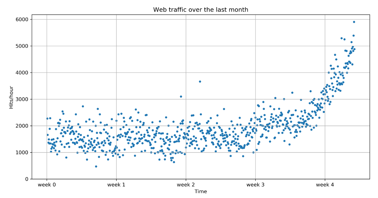
The main command here is plt.scatter(x, y, s=10), which plots the web traffic in y over the individual days in x. With s=10 we are setting the line width. Then we are dressing up the chart a bit (title, labels, grid, and so on) and finally we provide the possibility to add additional models to it.

You can run this function with the following:

>>> plot_web_traffic(x, y)

We will see what happens if you are in a Jupyter notebook session and have run the following command:

>>> %matplotlib inline

In one of the cells of the notebook, Jupyter will automatically show the generated graphs inline, using the following code:

>>> plot_web_traffic(x, y)

If you are in a normal command shell, you will have to save the graph to disk and then display it later with an image viewer:

>>> plt.savefig("web_traffic.png"))

In the resulting chart, we can see that while in the first weeks the traffic stayed more or less the same, the last week shows a steep increase:

Now that we have a first impression of the data, we return to the initial question: how long will our server be able to handle the incoming web traffic? To answer this, we have to do the following:

1. Find the real model behind the noisy data points
2. Use the model to find the point in time where our infrastructure won't handle the load anymore and has to be extended

When we talk about models, you can think of them as simplified theoretical approximations of complex reality. As such, there is always some inferiority involved, also called the approximation error. This error will guide us in choosing the right model among the many choices we have. We will calculate this error as the squared distance of the model's prediction to the real data; for example, for a learned model function, f, the error is calculated as follows:

def error(f, x, y):
    return np.sum((f(x)-y)**2)

The vectors x and y contain the web stats data that we extracted earlier. It is the beauty of NumPy's vectorized functions, which we exploit here with f(x). The trained model is assumed to take a vector and return the results again as a vector of the same size so that we can use it to calculate the difference to y.

Let's assume for a second that the underlying model is a straight line. Then the challenge is how to best put that line into the chart so that it results in the smallest approximation error. SciPy's polyfit() function does exactly that. Given data x and y and the desired order of the polynomial (a straight line has an order of 1), it finds the model function that minimizes the error function defined earlier:

fp1 = np.polyfit(x, y, 1)

The polyfit() function returns the parameters of the fitted Model function, fp1:

>>> print("Model parameters: %s" % fp1)
Model parameters: [ 2.59619213 989.02487106]

This means the best straight line fit is the following function:

f(x) = 2.59619213 * x + 989.02487106

We then use poly1d() to create a model function from the model parameters:

>>> f1 = np.poly1d(fp1)
>>> print(error(f1, x, y)) 
317389767.34

We can now use f1() to plot our first trained model. We have already implemented plot_web_traffic in a way that lets us easily add additional models to plot. In addition, we pass a list of models, of which we currently have only one:

plot_web_traffic(x, y, [f1])

This will produce the following plot:

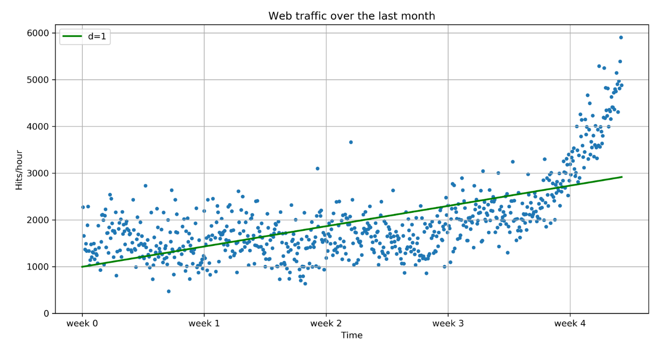
It seems like the first four weeks are not that far off, although we can clearly see that there is something wrong with our initial assumption that the underlying model is a straight line. Also, how good or how bad actually is the error of 319,531,507.008 ?

The absolute value of the error is seldom of use in isolation. However, when comparing two competing models, we can use their errors to judge which one of them is better. Although our first model clearly is not the one we would use, it serves a very important purpose in the workflow. We will use it as our baseline until we find a better one. Whatever model we come up with in the future, we will compare it against the current baseline.

Let's now fit a more complex model, a polynomial of degree 2, to see whether it better understands our data:

>>> f2p = np.polyfit(x, y, 2)
>>> print(f2p)
[ 1.05605675e-02 -5.29774287e+00 1.98466917e+03]
>>> f2 = np.poly1d(f2p)
>>> print(error(f2, x, y))
181347660.764

With plot_web_traffic(x, y, [f1, f2]) we can see how a function of degree 2 manages to model our web traffic data:

The error is 181,347,660.764, which is almost half the error of the straight-line model. This is good, but unfortunately this comes at a price: we now have a more complex function, meaning that we have one more parameter to tune inside polyfit(). The fitted polynomial is as follows:

f(x) = 0.0105605675 * x**2 - 5.29774287 * x + 1984.66917

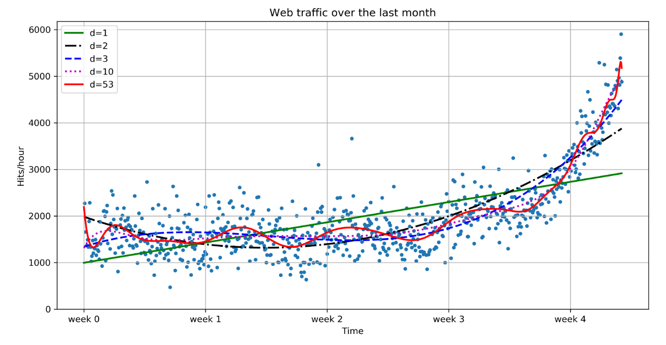
So, if more complexity gives better results, why not increase the complexity even more? Let's try it for degrees 3, 10, and 100:

Interestingly, we do not see d = 100 for the polynomial that had been fitted with 100 degrees, but instead d = 53. This has to do with the warning we get when fitting 100 degrees:

RankWarning: Polyfit may be poorly conditioned

This means that, because of numerical errors, polyfit cannot determine a good fit with 100 degrees. Instead, it figured that 53 would be good enough.

It seems like the curves capture the fitted data better the more complex they get. The errors seem to tell the same story:

>>> print("Errors for the complete data set:")
>>> for f in [f1, f2, f3, f10, f100]:
...     print("td=%i: %f" % (f.order, error(f, x, y)))
...

The errors for the complete dataset are as follows:

• d=1: 319,531,507.008126
• d=2: 181,347,660.764236
• d=3: 140,576,460.879141
• d=10: 123,426,935.754101
• d=53: 110,768,263.808878

However, taking a closer look at the fitted curves, we start to wonder whether they also capture the true process that generated that data. Framed differently, do our models correctly represent the underlying mass behavior of customers visiting our website? Looking at the polynomials of degree 10 and 53, we see wildly oscillating behavior. It seems that the models are fitted too much to the data. So much so that the graph is now capturing not only the underlying process, but also the noise. This is called overfitting.

At this point, we have the following choices:

• Choose one of the fitted polynomial models
• Switch to another more complex model class
• Think differently about the data and start again

Out of the five fitted models, the first-order model is clearly too simple, and the models of order 10 and 53 are clearly overfitting. Only the second- and third-order models seem to somehow match the data. However, if we extrapolate them at both borders, we see them going berserk.

Switching to a more complex class also doesn't seem to be the right way to go. Which arguments would back which class? At this point, we realize that we have probably not fully understood our data.

So, we step back and take another look at the data. It seems that there is an inflection point between weeks 3 and 4. Let's separate the data and train two lines using week 3.5 as a separation point:

>>> inflection = int(3.5*7*24) # calculate the inflection point in hours
>>> xa = x[:inflection] # data before the inflection point
>>> ya = y[:inflection]
>>> xb = x[inflection:] # data after
>>> yb = y[inflection:]

>>> fa = sp.poly1d(sp.polyfit(xa, ya, 1))
>>> fb = sp.poly1d(sp.polyfit(xb, yb, 1))

>>> fa_error = error(fa, xa, ya)
>>> fb_error = error(fb, xb, yb)
>>> print("Error inflection=%f" % (fa_error + fb_error))

Error inflection=132950348.197616

From the first line (straight), we train with the data up to week 3, and in the second line (dashed), we train with the remaining data:

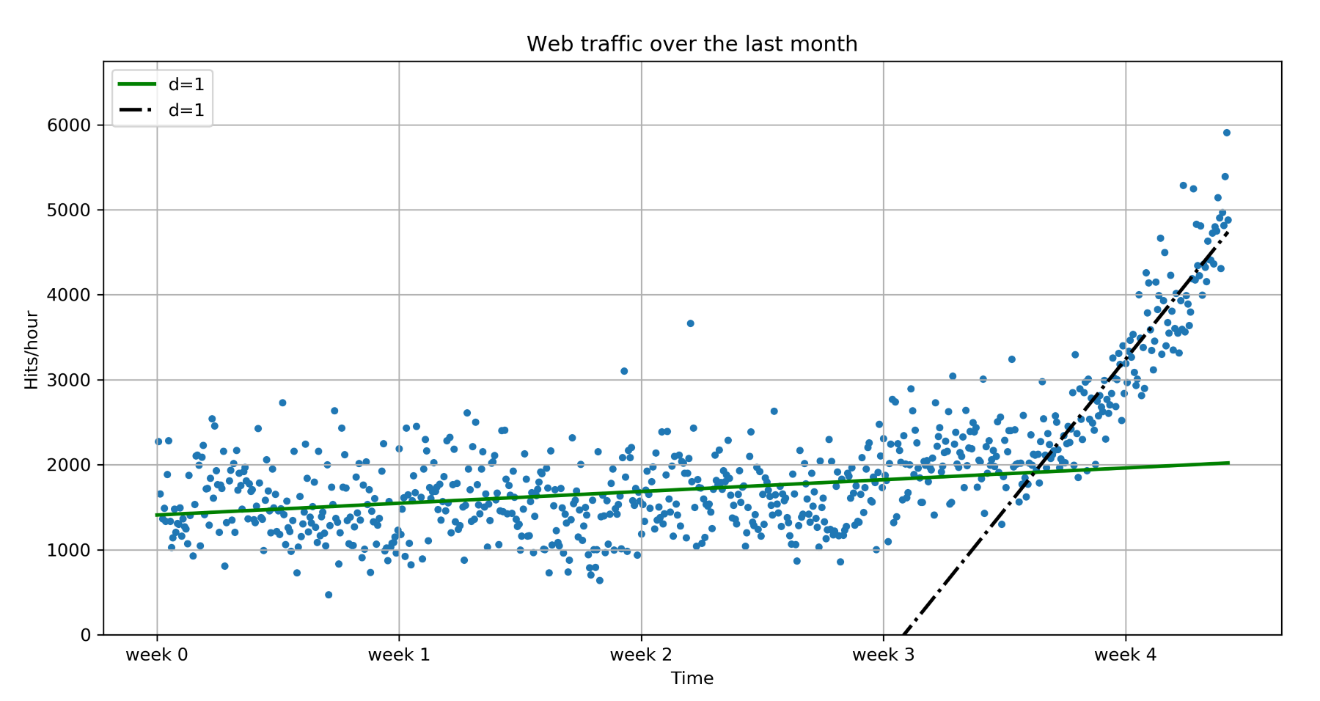
Clearly, the combination of these two lines seems to be a much better fit to the data than anything we have modeled before. But still, the combined error is higher than the higher order polynomials. Can we trust the error at the end?

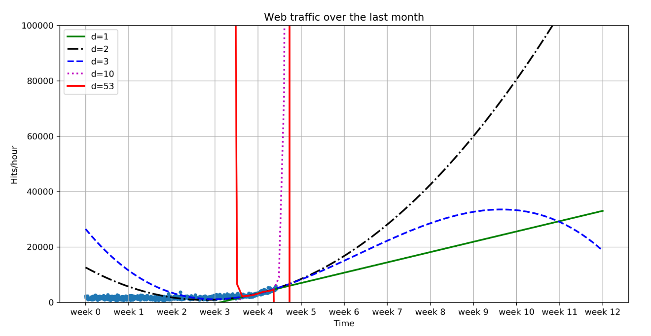
Asked differently, why do we trust the straight line fitted only during the last week of our data more than any of the more complex models? It is because we assume that it will capture future data better. If we plot the models into the future, we can see how right we are (d = 1 is again our initial straight line):

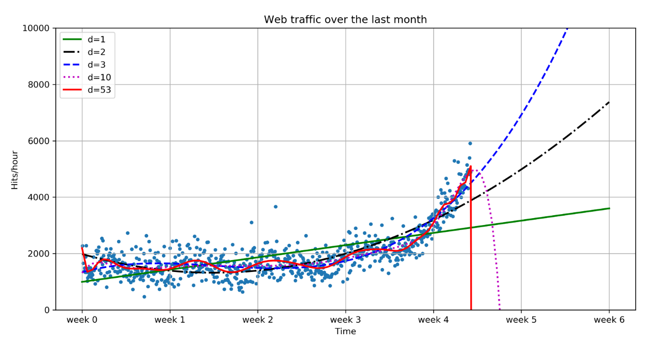
The models of degree 10 and 53 don't seem to expect a bright future of our start-up. They tried so hard to model the given data correctly that they are clearly useless to extrapolate beyond. This is called overfitting.

On the other hand, the lower degree models seem not to be capable of capturing the data well enough. This is called underfitting.

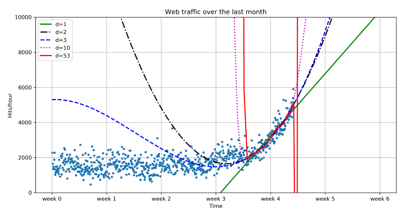
So, let's play fair to models of degree 2 and more and look at how they behave if we fit them only to the data of the last week. After all, we believe that the last week says more about the future than the data prior to it. The result can be seen in the following psychedelic chart, which further shows how bad the problem of overfitting is:

See following commands:

>>> fb1 = np.poly1d(np.polyfit(xb, yb, 1))
>>> fb2 = np.poly1d(np.polyfit(xb, yb, 2))
>>> fb3 = np.poly1d(np.polyfit(xb, yb, 3))
>>> fb10 = np.poly1d(np.polyfit(xb, yb, 10))
>>> fb100 = np.poly1d(np.polyfit(xb, yb, 100))

>>> print("Errors for only the time after inflection point")
>>> for f in [fb1, fb2, fb3, fb10, fb100]:
...    print("td=%i: %f" % (f.order, error(f, xb, yb)))

>>> plot_web_traffic(x, y, [fb1, fb2, fb3, fb10, fb100],
...     mx=np.linspace(0, 6 * 7 * 24, 100),
...     ymax=10000)

Following table shows errors and time after inflection point:

Still, judging from the errors of the models when trained only on the data from week 3.5 and later, we should still choose the most complex one (note that we also calculate the error when trained only on datapoints that occur after the inflection point).

If we only had some data from the future that we could use to measure our models against, then we should be able to judge our model choice only on the resulting approximation error.

Although we cannot look into the future, we can and should simulate a similar effect by holding out a part of our data. Let's remove, for instance, a certain percentage of the data and train on the remaining one. Then, we use the held-out data to calculate the error. As the model has been trained without knowing the held-out data, we should get a more realistic picture of how the model will behave in the future.

The test errors for the models trained only on the time after the inflection point now show a completely different picture:

• d=1: 6492812.705336
• d=2: 5008335.504620
• d=3: 5006519.831510
• d=10: 5440767.696731
• d=53: 5369417.148129

Have a look at the following plot:

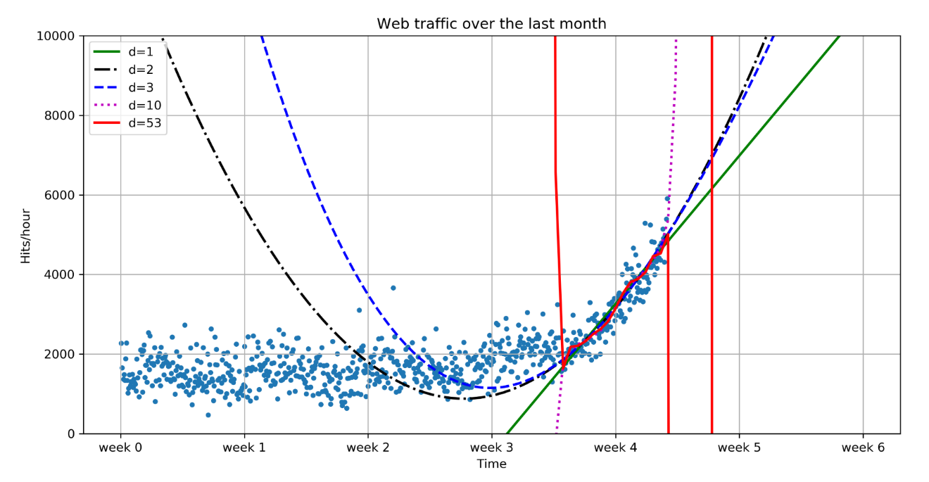
It seems the model with the degrees 2 and 3 has the lowest test error, which is the error that is shown when measured using data that the model did not see during training. This gives us hope that we won't get bad surprises when future data arrives. However, we are not fully done yet.

We will see in the next plot why we cannot simply pick the model with the lowest error:

The model with degree 3 does not foresee a future in which we will ever get 100,000 hits per hour. So we stick with degree 2.

We have finally arrived at some models that we think can represent the underlying process best. It is now a simple matter of finding out when our infrastructure will reach 100,000 requests per hour. We have to calculate when our model function reaches the value of 100,000. Because both models (degree 2 and 3) were so close together, we will do it for both.

With a polynomial of degree 2, we could simply compute the inverse of the function and calculate its value at 100,000. Of course, we would like to have an approach that is easily applicable to any model function.

This can be done by subtracting 100,000 from the polynomial, which results in another polynomial, and finding its root. SciPy's optimize module has the fsolve function to achieve this, when provided an initial starting position with the x0 parameter. As every entry in our input data file corresponds to one hour, and we have 743 of them, we set the starting position to some value after that. Let fbt2 be the winning polynomial of degree 2:

>>> fbt2 = np.poly1d(np.polyfit(xb[train], yb[train], 2))
>>> print("fbt2(x)= n%s" % fbt2) 
fbt2(x)=
         2
0.05404 x - 50.39 x + 1.262e+04

>>> print("fbt2(x)-100,000= n%s" % (fbt2-100000)) 
fbt2(x)-100,000=
         2
0.05404 x - 50.39 x - 8.738e+04

>>> from scipy.optimize import fsolve
>>> reached_max = fsolve(fbt2-100000, x0=800)/(7*24)

>>> print("100,000 hits/hour expected at week %f" % reached_max[0]) 
100,000 hits/hour expected at week 10.836350

It is expected to have 100,000 hits/hour at week 10.836350, so our model tells us that, given the current user behavior and traction of our start-up, it will take a couple more weeks for us to reach our capacity threshold.

Of course, there is a certain uncertainty involved with our prediction. To get a real picture of it, one could draw in more sophisticated statistics to find the variance we can expect when looking further and further into the future.

There are also the user and underlying user behavior dynamics that we cannot model accurately. However, at this point, we are fine with the current prediction as it is good enough to answer our initial question of when we would have to increase the capacity of our system. If we then monitor our web traffic closely, we will see in time when we have to allocate new resources.

Congratulations! You just learned two important things, of which the most important is that, as a typical machine learning operator, you will spend most of your time understanding and refining the data—exactly what we just did in our first, tiny machine learning example. We hope that this example helped you to start switching your mental focus from algorithms to data.

Then, you learned how important it is to have the correct experiment setup, and that it is vital to not mix up training and testing. Admittedly, the use of polynomial fitting is not the coolest thing in the machine learning world; we chose it so that you would not be distracted by the coolness of some shiny algorithm when we conveyed those two most important messages we mentioned earlier.

So, let's move on to Chapter 2, Classifying with Real-world Examples, we are on the topic of classification. Now, we will apply the concepts on a very specific, but very important, type of data, namely text.