The leaflet package is the de facto package for creating interactive maps in R. Part of its success is due to the fact that it works really well in conjunction with Shiny. Shiny is used to create interactive web interfaces in R, that can be accessed from any browser.

In order to run this recipe, you need to install the leaflet and dplyr packages using the install.packages() command.

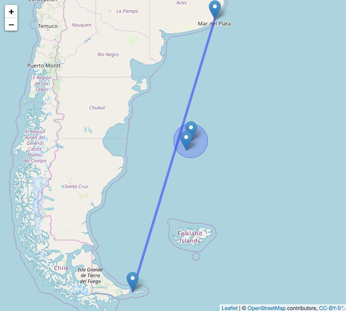
On November 15, 2017, a submarine from the Argentine Navy was lost in the South Atlantic Ocean along with its crew. It is suspected that a catastrophic accident occurred, that caused an explosion and later an implosion. The submarine departed from Ushuaia (South Argentina) and was expected to arrive at its headquarters in Mar del Plata (Central Argentina) navigating on a south-north trajectory. Its last contact was recorded circa -46.7333, -60.133 (when around 50% of its route had been covered), and a sound anomaly was later detected by hydrophones and triangulated at -46.12, -59.69. This anomaly happened a few hours after the submarine's last contact, and was consistent with an explosion. In November 2018, the submarine was found using several remotely operated underwater vehicles (ROVs) very near to the sound anomaly's position at around 900 meters depth.

In this recipe, we will first plot a line connecting its departure and destination ports. We will then add two markers—one for its last known position, and another one for the sound anomaly position. We will finally add a circle around this anomaly's position, indicating the area where most of the search efforts were concentrated.

1. Load the libraries:

library(dplyr)
library(leaflet)

2. We use two DataFrames—one for the line, and another one for the markers:

line = data.frame(lat = c(-54.777255,-38.038561),long=c(-64.936853,-57.529756),mag="start")
sub_data = data.frame(lat = c(-54.777255,-38.038561,-46.12,-46.73333333333333),long=c(-64.936853,-57.529756,-59.69,-60.13333333333333),mag=c("start","end","sound anomaly","last known position"))
area_search = data.frame(lat=-46.12,long=-59.69)

3. Plot the map with the line, the markers, and also a circle:

leaflet(data = sub_data) %>% addTiles() %>%
 addMarkers(~long, ~lat, popup = ~as.character(mag), label = ~as.character(mag)) %>%
 addPolylines(data = line, lng = ~long, lat = ~lat) %>% addCircles(lng = -59.69, lat = -46.12, weight = 1,radius = 120000)

The following screenshot shows the map and trajectory:

The leaflet package renders the map, along with the markers that we are passing through the sub_data DataFrame. The line is drawn using the addPolylines function. And the circle is drawn using the addCircles function.