Linear regression refers to finding the underlying function with the help of linear combination of input variables. The previous example had an input variable and an output variable. A simple linear regression is easy to understand, but represents the basis of regression techniques. Once these concepts are understood, it will be easier for us to address the other types of regression.

Consider the following diagram:

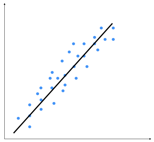
The linear regression method consists of precisely identifying a line that is capable of representing point distribution in a two-dimensional plane, that is, if the points corresponding to the observations are near the line, then the chosen model will be able to describe the link between the variables effectively.

In theory, there are an infinite number of lines that may approximate the observations, while in practice, there is only one mathematical model that optimizes the representation of the data. In the case of a linear mathematical relationship, the observations of the y variable can be obtained by a linear function of the observations of the x variable. For each observation, we will use the following formula:

In the preceding formula, x is the explanatory variable and y is the response variable. The α and β parameters, which represent the slope of the line and the intercept with the y-axis respectively, must be estimated based on the observations collected for the two variables included in the model.

The slope, α, is of particular interest, that is, the variation of the mean response for every single increment of the explanatory variable. What about a change in this coefficient? If the slope is positive, the regression line increases from left to right, and if the slope is negative, the line decreases from left to right. When the slope is zero, the explanatory variable has no effect on the value of the response. But it is not just the sign of α that establishes the weight of the relationship between the variables. More generally, its value is also important. In the case of a positive slope, the mean response is higher when the explanatory variable is higher, while in the case of a negative slope, the mean response is lower when the explanatory variable is higher.

The main aim of linear regression is to get the underlying linear model that connects the input variable to the output variable. This in turn reduces the sum of squares of differences between the actual output and the predicted output using a linear function. This method is called ordinary least squares. In this method, the coefficients are estimated by determining numerical values that minimize the sum of the squared deviations between the observed responses and the fitted responses, according to the following equation:

This quantity represents the sum of the squares of the distances to each experimental datum (x_i, y_i) from the corresponding point on the straight line.

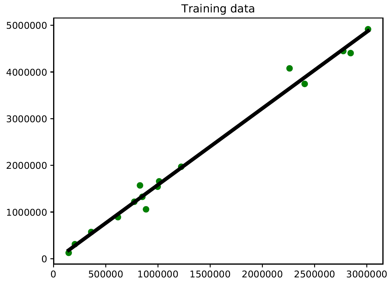
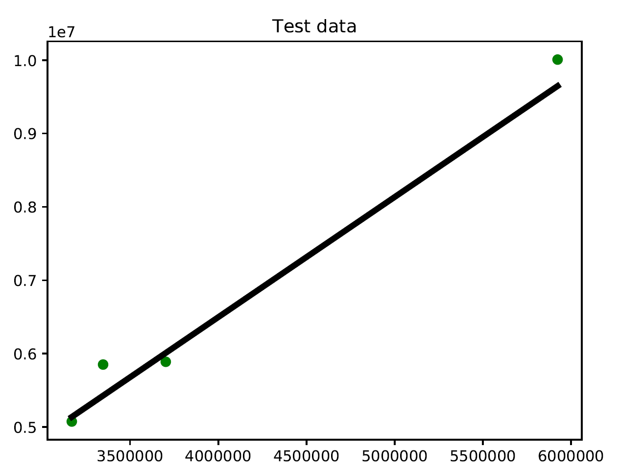
You might say that there might be a curvy line out there that fits these points better, but linear regression doesn't allow this. The main advantage of linear regression is that it's not complex. If you go into non-linear regression, you may get more accurate models, but they will be slower. As shown in the preceding diagram, the model tries to approximate the input data points using a straight line. Let's see how to build a linear regression model in Python.

Regression is used to find out the relationship between input data and the continuously-valued output data. This is generally represented as real numbers, and our aim is to estimate the core function that calculates the mapping from the input to the output. Let's start with a very simple example. Consider the following mapping between input and output:

1 --> 2
3 --> 6
4.3 --> 8.6
7.1 --> 14.2

If I ask you to estimate the relationship between the inputs and the outputs, you can easily do this by analyzing the pattern. We can see that the output is twice the input value in each case, so the transformation would be as follows:

This is a simple function, relating the input values with the output values. However, in the real world, this is usually not the case. Functions in the real world are not so straightforward!

You have been provided with a data file called VehiclesItaly.txt. This contains comma-separated lines, where the first element is the input value and the second element is the output value that corresponds to this input value. Our goal is to find the linear regression relation between the vehicle registrations in a state and the population of a state. You should use this as the input argument. As anticipated, the Registrations variable contains the number of vehicles registered in Italy and the Population variable contains the population of the different regions.

Let's see how to build a linear regressor in Python:

1. Create a file called regressor.py and add the following lines:

filename = "VehiclesItaly.txt"
X = []
y = []
with open(filename, 'r') as f:
    for line in f.readlines():
        xt, yt = [float(i) for i in line.split(',')]
        X.append(xt)
        y.append(yt)

We just loaded the input data into X and y, where X refers to the independent variable (explanatory variables) and y refers to the dependent variable (response variable). Inside the loop in the preceding code, we parse each line and split it based on the comma operator. We then convert them into floating point values and save them in X and y.

2. When we build a machine learning model, we need a way to validate our model and check whether it is performing at a satisfactory level. To do this, we need to separate our data into two groups—a training dataset and a testing dataset. The training dataset will be used to build the model, and the testing dataset will be used to see how this trained model performs on unknown data. So, let's go ahead and split this data into training and testing datasets:

num_training = int(0.8 * len(X))
num_test = len(X) - num_training

import numpy as np

# Training data
X_train = np.array(X[:num_training]).reshape((num_training,1))
y_train = np.array(y[:num_training])

# Test data
X_test = np.array(X[num_training:]).reshape((num_test,1))
y_test = np.array(y[num_training:])

First, we have put aside 80% of the data for the training dataset and the remaining 20% is for the testing dataset. Then, we have built four arrays: X_train, X_test,y_train, and y_test.

3. We are now ready to train the model. Let's create a regressor object, as follows:

from sklearn import linear_model

# Create linear regression object
linear_regressor = linear_model.LinearRegression()

# Train the model using the training sets
linear_regressor.fit(X_train, y_train)

First, we have imported linear_model methods from the sklearn library, which are methods used for regression, wherein the target value is expected to be a linear combination of the input variables. Then, we have used the LinearRegression() function, which performs ordinary least squares linear regression. Finally, the fit() function is used to fit the linear model. Two parameters are passed—training data (X_train), and target values (y_train).

4. We just trained the linear regressor, based on our training data. The fit() method takes the input data and trains the model. To see how it all fits, we have to predict the training data with the model fitted:

y_train_pred = linear_regressor.predict(X_train)

5. To plot the outputs, we will use the matplotlib library as follows:

import matplotlib.pyplot as plt
plt.figure()
plt.scatter(X_train, y_train, color='green')
plt.plot(X_train, y_train_pred, color='black', linewidth=4)
plt.title('Training data')
plt.show()

When you run this in the Terminal, the following diagram is shown:

6. In the preceding code, we used the trained model to predict the output for our training data. This wouldn't tell us how the model performs on unknown data, because we are running it on the training data. This just gives us an idea of how the model fits on training data. Looks like it's doing okay, as you can see in the preceding diagram!
7. Let's predict the test dataset output based on this model and plot it, as follows:

y_test_pred = linear_regressor.predict(X_test)
plt.figure()
plt.scatter(X_test, y_test, color='green')
plt.plot(X_test, y_test_pred, color='black', linewidth=4)
plt.title('Test data')
plt.show()

When you run this in the Terminal, the following output is returned:

As you might expect, there's a positive association between a state's population and the number of vehicle registrations.

In this recipe, we looked for the linear regression relation between the vehicle registrations in a state and the population of a state. To do this we used the LinearRegression() function of the linear_model method of the sklearn library. After constructing the model, we first used the data involved in training the model to visually verify how well the model fits the data. Then, we used the test data to verify the results.

The best way to appreciate the results of a simulation is to display those using special charts. In fact, we have already used this technique in this section. I am referring to the chart in which we drew the scatter plot of the distribution with the regression line. In Chapter 5, Visualizing Data, we will see other plots that will allow us to check the model's hypotheses.

• Scikit-learn's official documentation of the sklearn.linear_model.LinearRegression() function: https://scikit-learn.org/stable/modules/generated/sklearn.linear_model.LinearRegression.html.
• Regression Analysis with R, Giuseppe Ciaburro, Packt Publishing.
• Linear regression: https://en.wikipedia.org/wiki/Linear_regression.
• Introduction to Linear Regression: http://onlinestatbook.com/2/regression/intro.html.