One of the main problems of linear regression is that it's sensitive to outliers. During data collection in the real world, it's quite common to wrongly measure output. Linear regression uses ordinary least squares, which tries to minimize the squares of errors. The outliers tend to cause problems because they contribute a lot to the overall error. This tends to disrupt the entire model.

Let's try to deepen our understanding of the concept of outliers: outliers are values that, compared to others, are particularly extreme (values that are clearly distant from the other observations). Outliers are an issue because they might distort data analysis results; more specifically, descriptive statistics and correlations. We need to find these in the data cleaning phase, however, we can also get started on them in the next stage of data analysis. Outliers can be univariate when they have an extreme value for a single variable, or multivariate when they have a unique combination of values for a number of variables. Let's consider the following diagram:

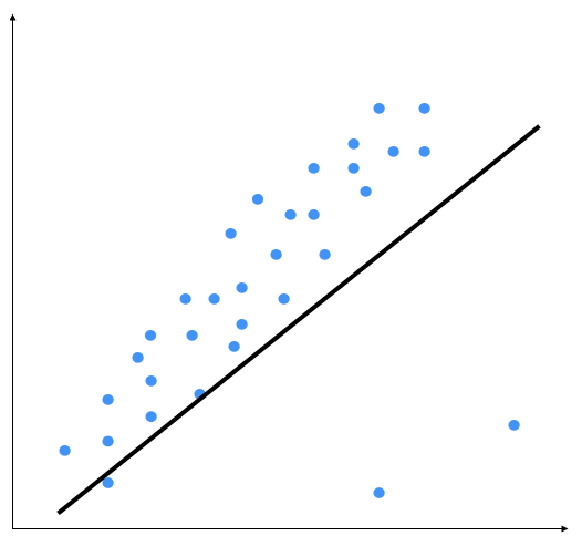
The two points on the bottom right are clearly outliers, but this model is trying to fit all the points. Hence, the overall model tends to be inaccurate. Outliers are the extreme values of a distribution that are characterized by being extremely high or extremely low compared to the rest of the distribution, and thus representing isolated cases with respect to the rest of the distribution. By visual inspection, we can see that the following output is a better model:

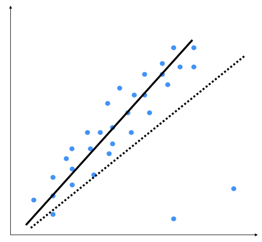
Ordinary least squares considers every single data point when it's building the model. Hence, the actual model ends up looking like the dotted line shown in the preceding graph. We can clearly see that this model is suboptimal.

The regularization method involves modifying the performance function, normally selected as the sum of the squares of regression errors on the training set. When a large number of variables are available, the least square estimates of a linear model often have a low bias but a high variance with respect to models with fewer variables. Under these conditions, there is an overfitting problem. To improve precision prediction by allowing greater bias but a small variance, we can use variable selection methods and dimensionality reduction, but these methods may be unattractive for computational burdens in the first case or provide a difficult interpretation in the other case.

Another way to address the problem of overfitting is to modify the estimation method by neglecting the requirement of an unbiased parameter estimator and instead considering the possibility of using a biased estimator, which may have smaller variance. There are several biased estimators, most of which are based on regularization: Ridge, Lasso, and ElasticNet are the most popular methods.

Ridge regression is a regularization method where a penalty is imposed on the size of the coefficients. As we said in the Building a linear regressor section, in the ordinary least squares method, the coefficients are estimated by determining numerical values that minimize the sum of the squared deviations between the observed responses and the fitted responses, according to the following equation:

Ridge regression, in order to estimate the β coefficients, starts from the basic formula of the residual sum of squares (RSS) and adds the penalty term. λ (≥ 0) is defined as the tuning parameter, which is multiplied by the sum of the β coefficients squared (excluding the intercept) to define the penalty period, as shown in the following equation:

It is evident that having λ = 0 means not having a penalty in the model, that is, we would produce the same estimates as the least squares. On the other hand, having a λ tending toward infinity means having a high penalty effect, which will bring many coefficients close to zero, but will not imply their exclusion from the model. Let's see how to build a ridge regressor in Python.

Let's see how to build a ridge regressor in Python:

1. You can use the data already used in the previous example: Building a linear regressor (VehiclesItaly.txt). This file contains two values in each line. The first value is the explanatory variable, and the second is the response variable.
2. Add the following lines to regressor.py. Let's initialize a ridge regressor with some parameters:

from sklearn import linear_model
ridge_regressor = linear_model.Ridge(alpha=0.01, fit_intercept=True, max_iter=10000)

3. The alpha parameter controls the complexity. As alpha gets closer to 0, the ridge regressor tends to become more like a linear regressor with ordinary least squares. So, if you want to make it robust against outliers, you need to assign a higher value to alpha. We considered a value of 0.01, which is moderate.
4. Let's train this regressor, as follows:

ridge_regressor.fit(X_train, y_train)
y_test_pred_ridge = ridge_regressor.predict(X_test)
print( "Mean absolute error =", round(sm.mean_absolute_error(y_test, y_test_pred_ridge), 2))
print( "Mean squared error =", round(sm.mean_squared_error(y_test, y_test_pred_ridge), 2))
print( "Median absolute error =", round(sm.median_absolute_error(y_test, y_test_pred_ridge), 2))
print( "Explain variance score =", round(sm.explained_variance_score(y_test, y_test_pred_ridge), 2))
print( "R2 score =", round(sm.r2_score(y_test, y_test_pred_ridge), 2))

Run this code to view the error metrics. You can build a linear regressor to compare and contrast the results on the same data to see the effect of introducing regularization into the model.

Ridge regression is a regularization method where a penalty is imposed on the size of the coefficients. Ridge regression is identical to least squares, barring the fact that ridge coefficients are computed by decreasing a quantity that is somewhat different. In ridge regression, a scale transformation has a substantial effect. Therefore, to avoid obtaining different results depending on the predicted scale of measurement, it is advisable to standardize all predictors before estimating the model. To standardize the variables, we must subtract their means and divide by their standard deviations.

• Scikit-learn's official documentation of the linear_model.Ridge function: https://scikit-learn.org/stable/modules/generated/sklearn.linear_model.Ridge.html
• Ridge Regression, Columbia University: https://www.mailman.columbia.edu/research/population-health-methods/ridge-regression
• Multicollinearity and Other Regression Pitfalls, The Pennsylvania State University: https://newonlinecourses.science.psu.edu/stat501/node/343/