Let's use a different regression method to solve the bicycle demand distribution problem. We will use the random forest regressor to estimate the output values. A random forest is a collection of decision trees. This basically uses a set of decision trees that are built using various subsets of the dataset, and then it uses averaging to improve the overall performance.

We will use the bike_day.csv file that is provided to you. This is also available at https://archive.ics.uci.edu/ml/datasets/Bike+Sharing+Dataset. There are 16 columns in this dataset. The first two columns correspond to the serial number and the actual date, so we won't use them for our analysis. The last three columns correspond to different types of outputs. The last column is just the sum of the values in the fourteenth and fifteenth columns, so we can leave those two out when we build our model. Let's go ahead and see how to do this in Python. We will analyze the code line by line to understand each step.

Let's see how to estimate bicycle demand distribution:

1. We first need to import a couple of new packages, as follows:

import csv
import numpy as np

2. We are processing a CSV file, so the CSV package for useful in handling these files. Let's import the data into the Python environment:

filename="bike_day.csv"
file_reader = csv.reader(open(filename, 'r'), delimiter=',')
X, y = [], []
for row in file_reader:
    X.append(row[2:13])
    y.append(row[-1])

This piece of code just read all the data from the CSV file. The csv.reader() function returns a reader object, which will iterate over lines in the given CSV file. Each row read from the CSV file is returned as a list of strings. So, two lists are returned: X and y. We have separated the data from the output values and returned them. Now we will extract feature names:

feature_names = np.array(X[0])

The feature names are useful when we display them on a graph. So, we have to remove the first row from X and y because they are feature names:

X=np.array(X[1:]).astype(np.float32)
y=np.array(y[1:]).astype(np.float32)

We have also converted the two lists into two arrays.

3. Let's shuffle these two arrays to make them independent of the order in which the data is arranged in the file:

from sklearn.utils import shuffle
X, y = shuffle(X, y, random_state=7)  

4. As we did earlier, we need to separate the data into training and testing data. This time, let's use 90% of the data for training and the remaining 10% for testing:

num_training = int(0.9 * len(X))
X_train, y_train = X[:num_training], y[:num_training]
X_test, y_test = X[num_training:], y[num_training:]

5. Let's go ahead and train the regressor:

from sklearn.ensemble import RandomForestRegressor
rf_regressor = RandomForestRegressor(n_estimators=1000, max_depth=10, min_samples_split=2)
rf_regressor.fit(X_train, y_train)

The RandomForestRegressor() function builds a random forest regressor. Here, n_estimators refers to the number of estimators, which is the number of decision trees that we want to use in our random forest. The max_depth parameter refers to the maximum depth of each tree, and the min_samples_split parameter refers to the number of data samples that are needed to split a node in the tree.

6. Let's evaluate the performance of the random forest regressor:

y_pred = rf_regressor.predict(X_test)
from sklearn.metrics import mean_squared_error, explained_variance_score
mse = mean_squared_error(y_test, y_pred)
evs = explained_variance_score(y_test, y_pred)
print( "#### Random Forest regressor performance ####")
print("Mean squared error =", round(mse, 2))
print("Explained variance score =", round(evs, 2))

The following results are returned:

#### Random Forest regressor performance ####
Mean squared error = 357864.36
Explained variance score = 0.89

7. Let's extract the relative importance of the features:

RFFImp= rf_regressor.feature_importances_ 
RFFImp= 100.0 * (RFFImp / max(RFFImp))
index_sorted = np.flipud(np.argsort(RFFImp))
pos = np.arange(index_sorted.shape[0]) + 0.5

To visualize the results, we will plot a bar graph:

import matplotlib.pyplot as plt
plt.figure()
plt.bar(pos, RFFImp[index_sorted], align='center')
plt.xticks(pos, feature_names[index_sorted])
plt.ylabel('Relative Importance')
plt.title("Random Forest regressor")
plt.show()

The following output is plotted:

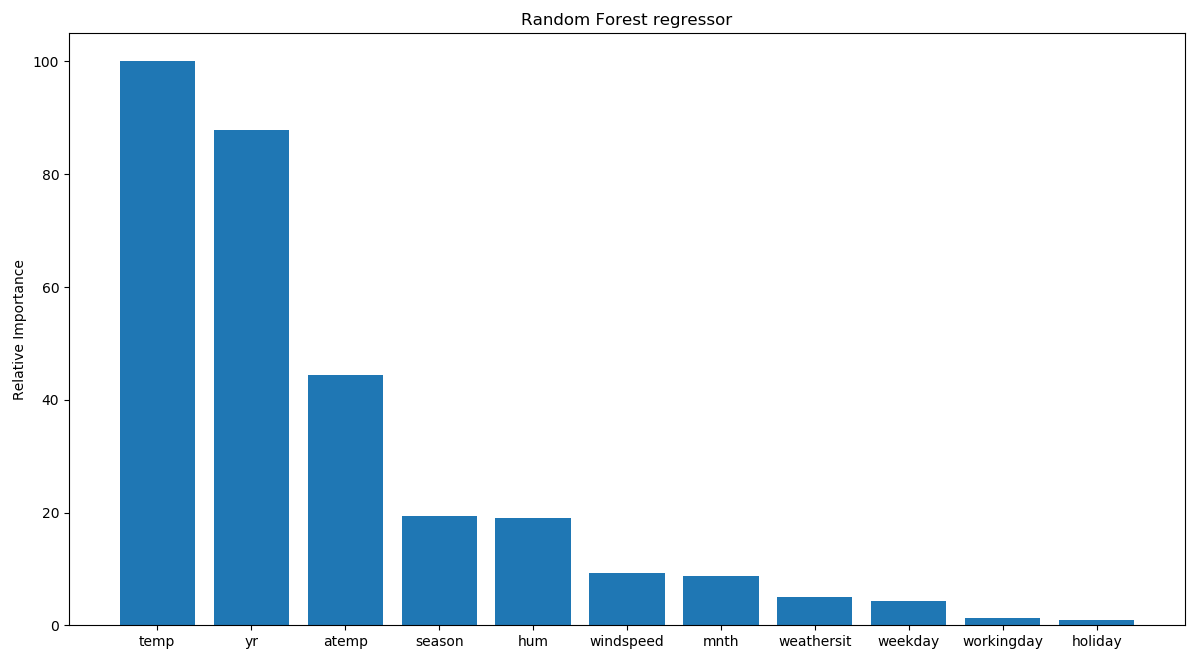
Looks like the temperature is the most important factor controlling bicycle rentals.

A random forest is a special regressor formed of a set of simple regressors (decision trees), represented as independent and identically distributed random vectors, where each one chooses the mean prediction of the individual trees. This type of structure has made significant improvements in regression accuracy and falls within the sphere of ensemble learning. Each tree within a random forest is constructed and trained from a random subset of the data in the training set. The trees therefore do not use the complete set, and the best attribute is no longer selected for each node, but the best attribute is selected from a set of randomly selected attributes.

Randomness is a factor that then becomes part of the construction of regressors and aims to increase their diversity and thus reduce correlation. The final result returned by the random forest is nothing but the average of the numerical result returned by the different trees in the case of a regression, or the class returned by the largest number of trees if the random forest algorithm was used to perform classification.

Let's see what happens when you include the fourteenth and fifteenth columns in the dataset. In the feature importance graph, every feature other than these two has to go to zero. The reason is that the output can be obtained by simply summing up the fourteenth and fifteenth columns, so the algorithm doesn't need any other features to compute the output. Make the following change inside the for loop (the rest of the code remains unchanged):

X.append(row[2:15])

If you plot the feature importance graph now, you will see the following:

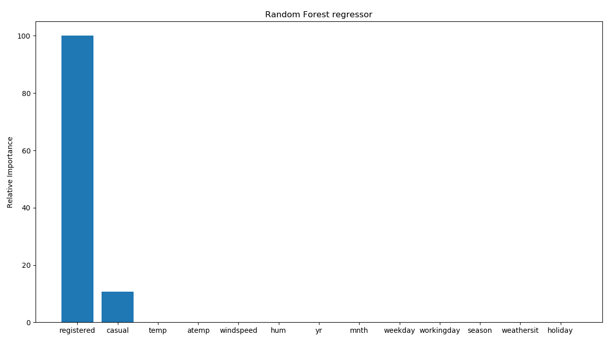
As expected, it says that only these two features are important. This makes sense intuitively because the final output is a simple summation of these two features. So, there is a direct relationship between these two variables and the output value. Hence, the regressor says that it doesn't need any other variable to predict the output. This is an extremely useful tool to eliminate redundant variables in your dataset. But this is not the only difference from the previous model. If we analyze the model's performance, we can see a substantial improvement:

#### Random Forest regressor performance ####
Mean squared error = 22552.26
Explained variance score = 0.99

We therefore have 99% of the variance explained: a very good result.

There is another file, called bike_hour.csv, that contains data about how the bicycles are shared hourly. We need to consider columns 3 to 14, so let's make this change in the code (the rest of the code remains unchanged):

filename="bike_hour.csv"
file_reader = csv.reader(open(filename, 'r'), delimiter=',')
X, y = [], []
for row in file_reader:
    X.append(row[2:14])
    y.append(row[-1])

If you run the new code, you will see the performance of the regressor displayed, as follows:

#### Random Forest regressor performance ####
Mean squared error = 2613.86
Explained variance score = 0.92

The feature importance graph will look like the following:

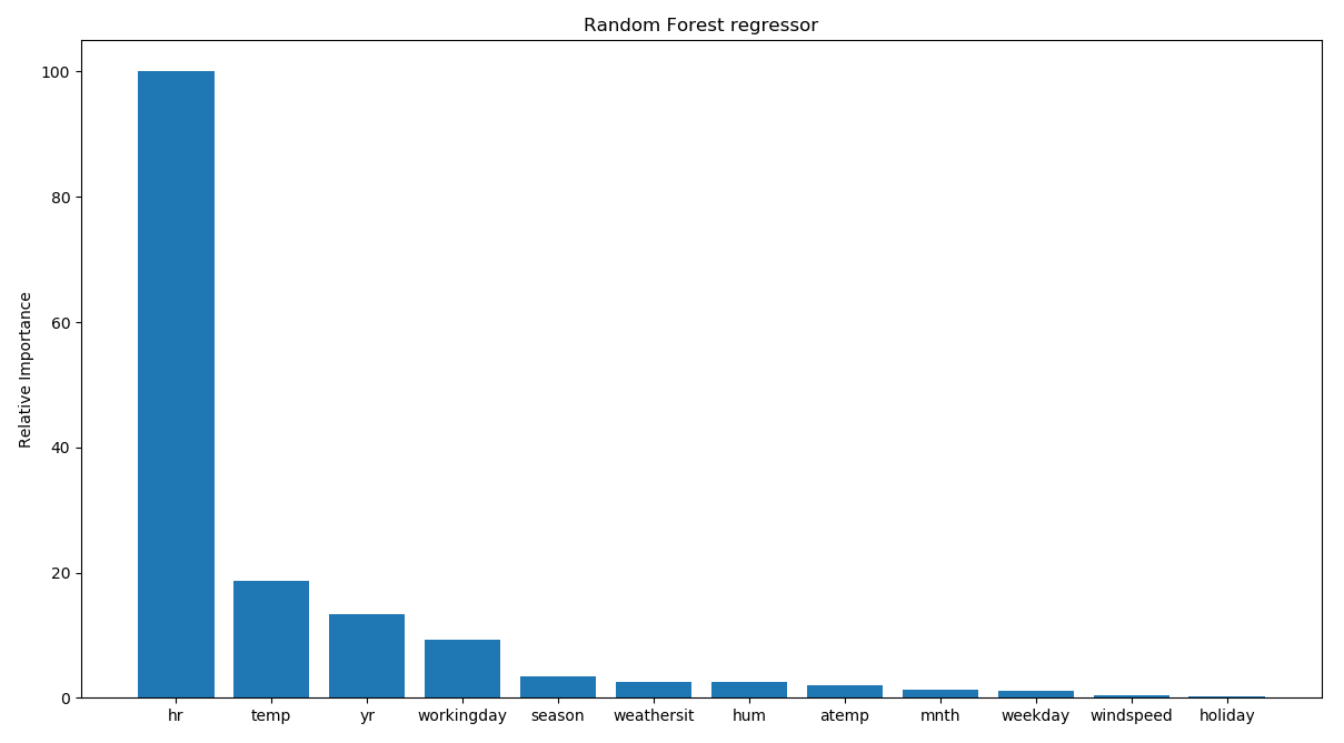
This shows that the hour of the day is the most important feature, which makes sense intuitively if you think about it! The next important feature is temperature, which is consistent with our earlier analysis.

• Scikit-learn's official documentation of the RandomForestRegressor function: https://scikit-learn.org/stable/modules/generated/sklearn.ensemble.RandomForestRegressor.html