
Hopefully, by now, you can see that finding clusters is extremely valuable in a machine learning workflow. However, how can you actually find these clusters? One of the most basic yet popular approaches is by using a cluster analysis called k-means clustering. k-means works by searching for K clusters in your data and the workflow is actually quite intuitive – we will start with the no-math introduction to k-means, followed by an implementation in Python.
Here is the no-math algorithm of k-means clustering:
Pick K centroids (K = expected distinct # of clusters).
Randomly place K centroids anywhere amongst your existing training data.
Calculate the Euclidean distance from each centroid to all the points in your training data.
Training data points get grouped in with their nearest centroid.
Amongst the data points grouped into each centroid, calculate the mean data point and move your centroid to that location.
Repeat this process until convergence, or when the membership in each group no longer changes.
And that's it! Here is the process laid out step-by-step with a simple cluster example:
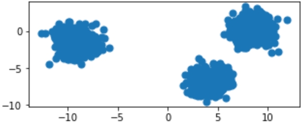
Figure 1.11: Original raw data charted on x,y coordinates
Provided with the original data in Figure 1.11, we can show the iterative process of k-means by showing the predicted clusters in each step:
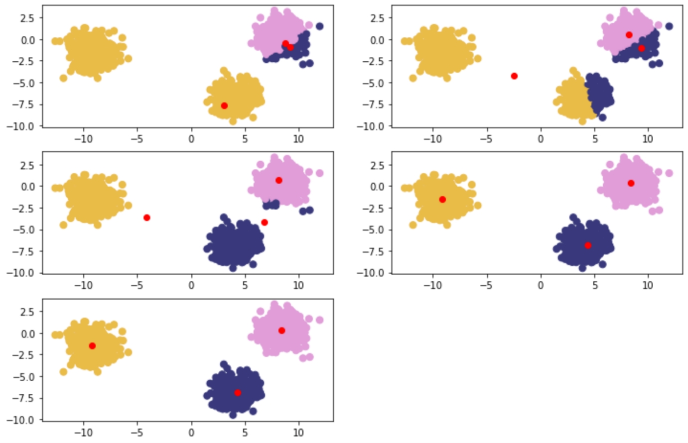
Figure 1.12: Reading from left to right – red points are randomly initialized centroids, and the closest data points are assigned to groupings of each centroid
To understand k-means at a deeper level, let's walk through the example given in the introductory section again with some of the math that supports k-means. The key component at play is the Euclidean distance formula:

Figure 1.13: Euclidean distance formula
Centroids are randomly set at the beginning as points in your n-dimensional space. Each of these centers is fed into the preceding formula as (a,b), and a point in your space is fed in as (x,y). Distances are calculated between each point and the coordinates of every centroid, with the centroid the shortest distance away chosen as the point's group.
The process is as follows:
Random Centroids: [ (2,5) , (8,3) , (4, 5) ]
Arbitrary point x: (0, 8)
Distance from point to each centroid: [ 3.61, 9.43, 5.00 ]
Point x is assigned to Centroid 1.
Euclidean distance is the most common distance metric for many machine learning applications and is often known colloquially as the distance metric; however, it is not the only, or even the best, distance metric for every situation. Another popular distance metric in use for clustering is Manhattan distance.
Manhattan distance is called as such because the intuition behind the metric is as though you were driving a car through a metropolis (such as New York City) that has many square blocks. Euclidean distance relies on diagonals due to it being based on Pythagorean theorem, while Manhattan distance constrains distance to only right angles. The formula for Manhattan distance is as follows:
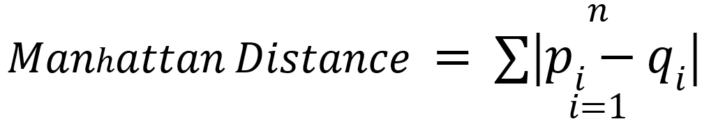
Figure 1.14: Manhattan distance formula
Here,  are vectors as in Euclidean distance. Building upon our examples of Euclidean distance, where we want to find the distance between two points, if
  and
and  , then the Manhattan distance would equal
  . This functionality scales to any number of dimensions. In practice, Manhattan distance may outperform Euclidean distance when it comes to higher dimensional data.
The preceding examples are clear to visualize when your data is only two-dimensional. This is for convenience, to help drive the point home of how k-means works and could lead you into a false understanding of how easy clustering is. In many of your own applications, your data will likely be orders of magnitude larger to the point that it cannot be perceived by visualization (anything beyond three dimensions will be imperceivable to humans). In the previous examples, you could mentally work out a few two-dimensional lines to separate the data into its own groups. At higher dimensions, you will need to be aided by a computer to find an n-dimensional hyperplane that adequately separates the dataset. In practice, this is where clustering methods such as k-means provide significant value.
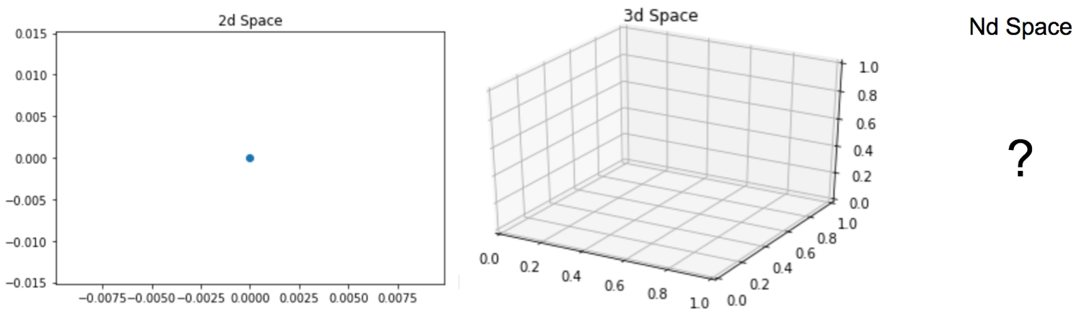
Figure 1.15: Two-dimensional, three-dimensional, and n-dimensional plots
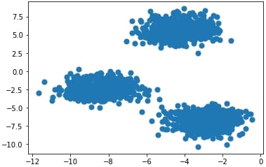
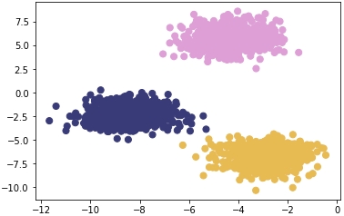
Figure 1.17: Plot of the coordinates with correct cluster labels
Figure 1.16: Plot of the coordinates
In the next exercise, we will calculate Euclidean distance. We will use the NumPy and Math packages. NumPy is a scientific computing package for Python that pre-packages common mathematical functions in highly-optimized formats. By using a package such as NumPy or Math, we help cut down the time spent creating custom math functions from scratch and instead focus on developing our solutions.
In this exercise, we will create an example point along with three sample centroids to help illustrate how Euclidean distance works. Understanding this distance formula is foundational to the rest of our work in clustering.
By the end of this exercise, we will be able to implement Euclidean distance from scratch and fully understand what it does to points in a feature space.
In this exercise, we will be using the standard Python built-in math package. There are no prerequisites for using the math package and it is included in all standard installations of Python. As the name suggests, this package is very useful, allowing to use a variety of basic math building blocks off the shelf, such as exponentials, square roots, and others:
Open a Jupyter notebook and create a naïve formula that captures the direct math of Euclidean distance, as follows:
import math
import numpy as np
def dist(a, b):
    return math.sqrt(math.pow(a[0]-b[0],2) + math.pow(a[1]-b[1],2))
This approach is considered naïve because it performs element-wise calculations on your data points (slow) compared to a more real-world implementation using vectors and matrix math to achieve significant performance increases.
Create the data points in Python as follows:
centroids = [ (2, 5), (8, 3), (4,5) ]
x = (0, 8)
Use the formula you created to calculate the Euclidean distance between the example point and each of the three centroids you were provided:
centroid_distances =[]
for centroid in centroids:
    centroid_distances.append(dist(x,centroid))
print(centroid_distances)
print(np.argmin(centroid_distances))
The output is as follows:
[3.605551275463989, 9.433981132056603, 5.0]
0
Since Python is zero-indexed, a position of zero as the minimum in our list of centroid distances signals to us that the example point, x, will be assigned to the number one centroid of three.
This process is repeated for every point in the dataset until each point is assigned to a cluster. After each point is assigned, the mean point is calculated among all of the points within each cluster. The calculation of the mean among these points is the same as calculating a mean between single integers.
Now that you have found clusters in your data using Euclidean distance as the primary metric, think back to how you did this easily in Exercise 2, Calculating Euclidean Distance in Python. It is very intuitive for our human minds to see groups of dots on a plot and determine which dots belong to discrete clusters. However, how do we ask a naïve computer to repeat this same task? By understanding this exercise, you help teach a computer an approach to forming clusters of its own with the notion of distance. We will build upon how we use these distance metrics in the next exercise.
By understanding this exercise, you'll help to teach a computer an approach to forming clusters of its own with the notion of distance. We will build upon how we use these distance metrics in this exercise:
Store the points [ (0,8), (3,8), (3,4) ] that are assigned to cluster one:
cluster_1_points =[ (0,8), (3,8), (3,4) ]
Calculate the mean point between all of the points to find the new centroid:
mean =[ (0+3+3)/3, (8+8+4)/3 ]
print(mean)
The output is as follows:
[2.0, 6.666666666666667]
After a new centroid is calculated, you will repeat the cluster membership calculation seen in Exercise 2, Calculating Euclidean Distance in Python, and then the previous two steps to find the new cluster centroid. Eventually, the new cluster centroid will be the same as the one you had entering the problem, and the exercise will be complete. How many times this repeats depends on the data you are clustering.
Once you have moved the centroid location to the new mean point of (2, 6.67), you can compare it to the initial list of centroids you entered the problem with. If the new mean point is different than the centroid that is currently in your list, that means you have to go through another iteration of the preceding two exercises. Once the new mean point you calculate is the same as the centroid you started the problem with, you have completed a run of k-means and reached a point called convergence.
In the next exercise, we will implement k-means from scratch.
In this exercise, we will have a look at the implementation of k-means from scratch. This exercise relies on scikit-learn, an open-source Python package that enables the fast prototyping of popular machine learning models. Within scikit-learn, we will be using the datasets functionality to create a synthetic blob dataset. In addition to harnessing the power of scikit-learn, we will also rely on Matplotlib, a popular plotting library for Python that makes it easy for us to visualize our data. To do this, perform the following steps:
Import the necessary libraries:
from sklearn.datasets import make_blobs
import matplotlib.pyplot as plt
import numpy as np
import math
%matplotlib inline
Generate a random cluster dataset to experiment on X = coordinate points, y = cluster labels, and define random centroids:
X, y = make_blobs(n_samples=1500, centers=3,
                  n_features=2, random_state=800)
centroids = [[-6,2],[3,-4],[-5,10]]
Print the data:
X
The output is as follows:
array([[-3.83458347,  6.09210705],
       [-4.62571831,  5.54296865],
       [-2.87807159, -7.48754592],
       ...,
        [-3.709726  , -7.77993633],
        [-8.44553266, -1.83519866],
        [-4.68308431,  6.91780744]])
Plot the coordinate points as follows:
plt.scatter(X[:, 0], X[:, 1], s=50, cmap='tab20b')
plt.show()
The plot looks as follows:
Print the array of y:
y
The output is as follows:
array([2, 2, 1, ..., 1, 0, 2])
Plot the coordinate points with the correct cluster labels:
plt.scatter(X[:, 0], X[:, 1], c=y,s=50, cmap='tab20b')
plt.show()
The plot looks as follows:
Let's recreate these results on our own! We will go over an example implementing this with some optimizations. This exercise is built on top of the previous exercise and should be performed in the same Jupyter notebook. For this exercise, we will rely on SciPy, a Python package that allows easy access to highly optimized versions of scientific calculations. In particular, we will be implementing Euclidean distance with cdist, the functionally of which replicates the barebones implementation of our distance metric in a much more efficient manner:
A non-vectorized implementation of Euclidean distance is as follows:
def dist(a, b):
    return math.sqrt(math.pow(a[0]-b[0],2) + math.pow(a[1]-b[1],2))
Now, implement the optimized Euclidean distance:
from scipy.spatial.distance import cdist
Store the values of X:
X[105:110]
The output is as follows:
array([[-3.09897933,  4.79407445],
       [-3.37295914, -7.36901393],
        [-3.372895  ,  5.10433846],
        [-5.90267987, -3.28352194],
        [-3.52067739,  7.7841276 ]])
Calculate the distances and choose the index of the shortest distance as a cluster:
for x in X[105:110]:
    calcs = []
    for c in centroids:
        calcs.append(dist(x, c))
    print(calcs, "Cluster Membership: ", np.argmin(calcs, axis=0))
Define the k_means function as follows and initialize k-centroids randomly. Repeat the process until the difference between new/old centroids equal 0 using the while loop:
def k_means(X, K):
    # Keep track of history so you can see k-means in action
    centroids_history = []
    labels_history = []
    rand_index = np.random.choice(X.shape[0], K)
    centroids = X[rand_index]
    centroids_history.append(centroids)
    while True:

# Euclidean distances are calculated for each point relative to
# centroids, and then np.argmin returns the index location of the
# minimal distance - which cluster a point is assigned to

        labels = np.argmin(cdist(X, centroids), axis=1)
        labels_history.append(labels)

    # Take mean of points within clusters to find new centroids

        new_centroids = np.array([X[labels == i].mean(axis=0)
                                  for i in range(K)])
        centroids_history.append(new_centroids)

# If old centroids and new centroids no longer change, k-means is
# complete and end. Otherwise continue

        if np.all(centroids == new_centroids):
            break
        centroids = new_centroids

    return centroids, labels, centroids_history, labels_history

centers, labels, centers_hist, labels_hist = k_means(X, 3)
Zip together the historical steps of centers and their labels:
for x, y in history:
    plt.figure(figsize=(4,3))
    plt.scatter(X[:, 0], X[:, 1], c=y, s=50, cmap='tab20b');
    plt.scatter(x[:, 0], x[:, 1], c='red')
As you can see in the above figures, k-means takes an iterative approach to refining optimal clusters based on distance. The algorithm starts with random initialization and depending on the complexity of the data, quickly finds the separations that make the most sense.
plt.show()
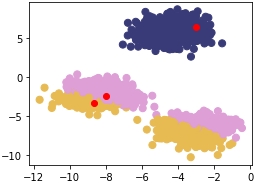
Figure 1.18: First scatterplot
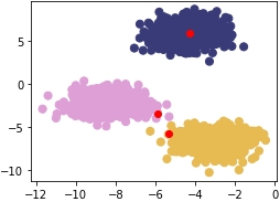
Figure 1.19: Second scatterplot
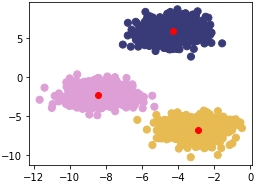
Figure 1.20: Third scatterplot
The first plot is as follows:
The second plot is as follows:
The third plot is as follows:
Understanding the performance of unsupervised learning methods is inherently much more difficult than supervised learning methods because, often, there is no clear-cut "best" solution. For supervised learning, there are many robust performance metrics – the most straightforward of these being accuracy in the form of comparing model-predicted labels to actual labels and seeing how many the model got correct. Unfortunately, for clustering, we do not have labels to rely on and need to build an understanding of how "different" our clusters are. We achieve this with the Silhouette Score metric. Inherent to this approach, we can also use Silhouette Scores to find optimal "K" numbers of clusters for our unsupervised learning methods.
The Silhouette metric works by analyzing how well a point fits within its cluster. The metric ranges from -1 to 1 – If the average silhouette score across your clustering is one, then you will have achieved perfect clusters and there will be minimal confusion about which point belongs where. If you think of the plots in our last exercise, the Silhouette score will be much closer to one, since the blobs are tightly condensed and there is a fair amount of distance between each blob. This is very rare though – the Silhouette Score should be treated as an attempt at doing the best you can, since hitting one is highly unlikely.
Mathematically, the Silhouette Score calculation is quite straightforward via the Simplified Silhouette Index (SSI), as 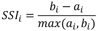 where
where  is the distance from point i to its own cluster centroid and
  is the distance from point i to the nearest cluster centroid.
The intuition captured here is that  represents how cohesive point i's cluster is as a clear cluster, and
  represents how far apart the clusters lie. We will use the optimized implementation of silhouette_score in scikit-learn for Activity 1, Implementing k-means Clustering. Using it is simple and only requires you to pass in the feature array and the predicted cluster labels from your k-means clustering method.
In the next exercise, we will use the pandas library to read a CSV. Pandas is a Python library that makes data wrangling easier through the use of DataFrames. To read data in Python, you will use variable_name = pd.read_csv('file_name.csv', header=None).
In this exercise, we're going to learn how to calculate the Silhouette Score of a dataset with a fixed number of clusters. For this, we will use the Iris dataset, which is available at https://github.com/TrainingByPackt/Unsupervised-Learning-with-Python/tree/master/Lesson01/Exercise06.
Note
This dataset was downloaded from https://archive.ics.uci.edu/ml/machine-learning-databases/iris/iris.data. It can be accessed at https://github.com/TrainingByPackt/Unsupervised-Learning-with-Python/tree/master/Lesson01/Exercise06.
Load the Iris data file using pandas, a package that makes data wrangling much easier through the use of DataFrames:
import pandas as pd
import numpy as np
import matplotlib.pyplot as plt
from sklearn.metrics import silhouette_score
from scipy.spatial.distance import cdist
iris = pd.read_csv('iris_data.csv', header=None)
iris.columns = ['SepalLengthCm', 'SepalWidthCm', 'PetalLengthCm', 'PetalWidthCm', 'species']
Separate the X features, since we want to treat this as an unsupervised learning problem:
X = iris[['SepalLengthCm', 'SepalWidthCm', 'PetalLengthCm', 'PetalWidthCm']]
Bring back the k_means function we made earlier for reference:
def k_means(X, K):
#Keep track of history so you can see k-means in action
    centroids_history = []
    labels_history = []
    rand_index = np.random.choice(X.shape[0], K)
    centroids = X[rand_index]
    centroids_history.append(centroids)
    while True:
# Euclidean distances are calculated for each point relative to
# centroids, #and then np.argmin returns
# the index location of the minimal distance - which cluster a point
# is #assigned to
        labels = np.argmin(cdist(X, centroids), axis=1)
        labels_history.append(labels)
#Take mean of points within clusters to find new centroids:
        new_centroids = np.array([X[labels == i].mean(axis=0)
                                  for i in range(K)])
        centroids_history.append(new_centroids)

# If old centroids and new centroids no longer change, k-means is
# complete and end. Otherwise continue
        if np.all(centroids == new_centroids):
            break
        centroids = new_centroids

    return centroids, labels, centroids_history, labels_history
Convert our Iris X feature DataFrame to a NumPy matrix:
X_mat = X.values
Run our k_means function on the Iris matrix:
centroids, labels, centroids_history, labels_history = k_means(X_mat, 3)
Calculate the Silhouette Score for the PetalLengthCm and PetalWidthCm columns:
silhouette_score(X[['PetalLengthCm','PetalWidthCm']], labels)
The output is similar to:
0.6214938502379446
In this exercise, we calculated the Silhouette Score for the PetalLengthCm and PetalWidthCm columns of the Iris dataset.