

Introduction to R
R provides an extensive set of libraries for visualization, data manipulation, statistical analysis, and model building. We will check the installation of R, perform some visualization, and build models in RStudio.
To test if the installation is successful, write this simple command as follows:
print("Hi")
The output is as follows:
"Hi"
After installing R, let's write the first R script in RStudio.
Exercise 1: Reading from a CSV File in RStudio
In this exercise, we will set the working directory and then read from an existing CSV file:
- We can set any directory containing all our code as the working directory so that we need not give the full path to access the data from that folder:
# Set the working directory
setwd("C:/R")
- Write an R script to load data into data frames:
data = read.csv("mydata.csv")
data
The output is as follows:
Col1 Col2 Col3
1 1 2 3
2 4 5 6
3 7 8 9
4 a b c
Other functions that are used to read files are read.table(), read.csv2(), read.delim(), and read.delim2().
R scripts are simple to write. Let's move on to operations in R.
Exercise 2: Performing Operations on a Dataframe
In this exercise, we will display the values of a column in the dataframe and also add a new column with values into the dataframe using the rbind() and cbind() functions.
- Let's print Col1 values using the dataframe["ColumnName"] syntax:
data['Col1']
Col1
The output is as follows:
1 1
2 4
3 7
4 a
- Create a new column Col4 using cbind() function. This is similar to rbind():
cbind(data,Col4=c(1,2,3,4))
The output is as follows:
Col1 Col2 Col3 Col4
1 1 2 3 1
2 4 5 6 2
3 7 8 9 3
4 a b c 4
- Create a new row in the dataframe using the rbind() function:
rbind(data,list(1,2,3))
The output is as follows:
Col1 Col2 Col3
1 1 2 3
2 4 5 6
3 7 8 9
4 a b c
5 1 2 3
We have added columns to the dataframe using the rbind() and cbind() functions. We will move ahead to understanding how exploratory data analysis helps us understand the data better.
Exploratory Data Analysis (EDA)
Exploratory Data Analysis (EDA) is the use of visualization techniques to explore the dataset. We will use the built-in dataset in R to learn to see a few statistics about the data. The datasets used are as follows:
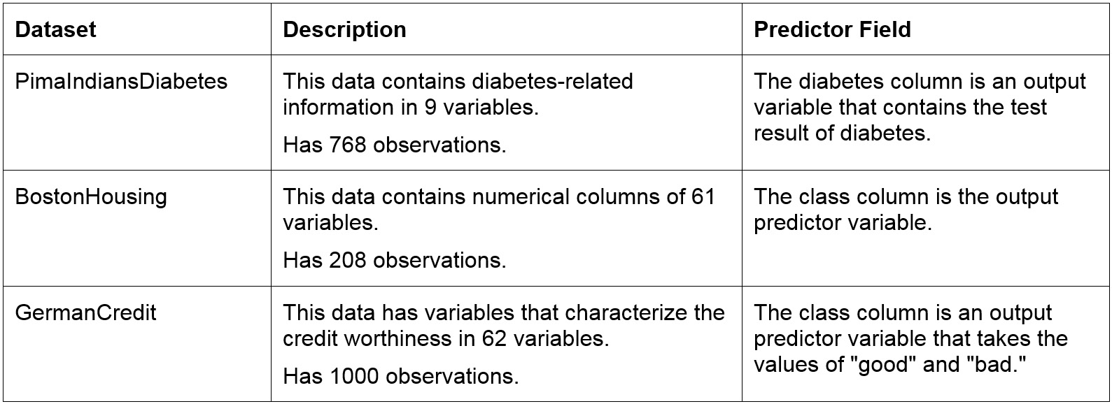
Figure 1.4: Datasets and their descriptions
View Built-in Datasets in R
To install packages to R, we use the following syntax: install.packages("Name_of_package")
The pre-loaded datasets of R can be viewed using the data() command:
#Installing necessary packages
install.packages("mlbench")
install.packages("caret")
#Loading the datasets
data(package = .packages(all.available = TRUE))
The datasets will be displayed in the dataset tab as follows:
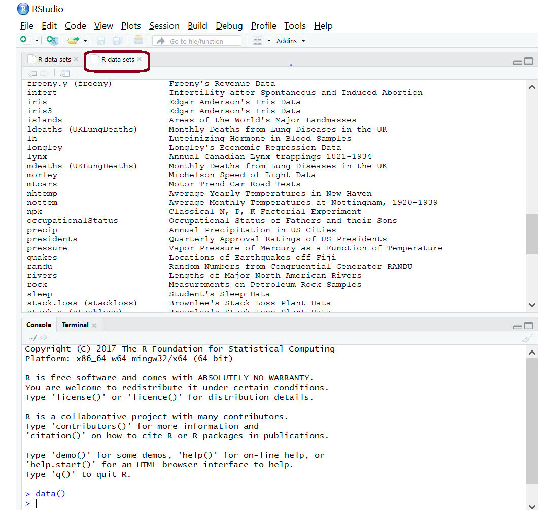
Figure 1.5: Dataset tab for viewing all the datasets
We can thus install packages and load the built-in datasets.
Exercise 3: Loading Built-in Datasets
In this exercise, we will load built-in datasets, analyze the contents of the datasets, and read the first and last records from those datasets.
- We will use the BostonHousing and GermanCredit datasets shown in the following screenshot:
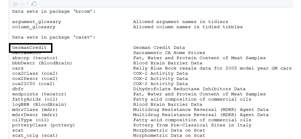
Figure 1.6: The GermanCredit dataset
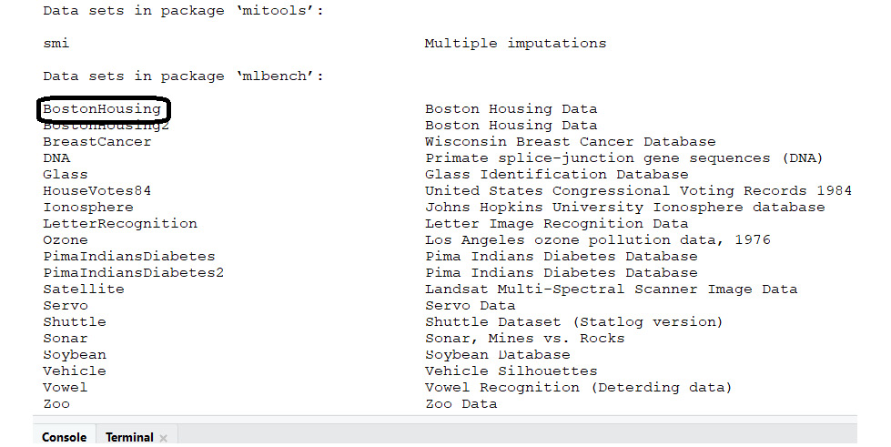
Figure 1.7: The BostonHousing dataset
- Check the installed packages using the following code:
data(package = .packages(all.available = TRUE))
- Choose File | New File | R Script:
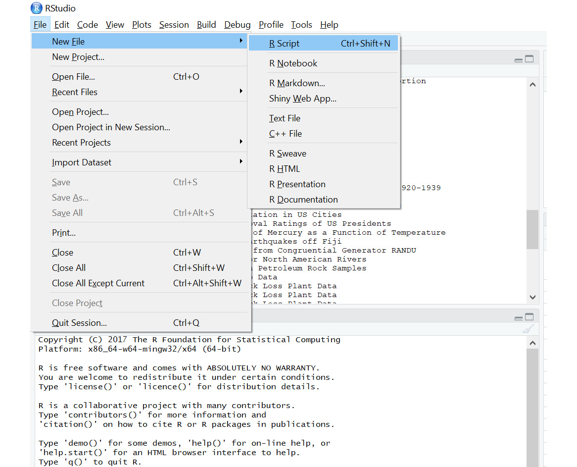
Figure 1.8: A new R script window
- Save the file into the local directory by clicking Ctrl + S on windows.
- Load the mlbench library and the BostonHousing dataset:
library(mlbench)
#Loading the Data
data(BostonHousing)
- The first five rows in the data can be viewed using the head() function, as follows:
#Print the first 5 lines in the dataset
head(BostonHousing)
- Click the Run option as shown:
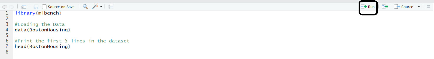
Figure 1.9: The Run option
The output will be as follows:
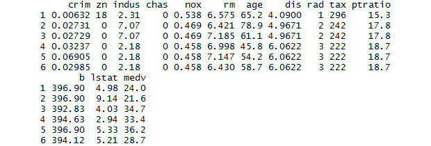
Figure 1.10: The first rows of Boston Housing dataset
- The description of the dataset can be viewed using <<Dataset>>. In place of <<Dataset>>, mention the name of the dataset:
# Display information about Boston Housing dataset
?BostonHousing
The Help tab will display all the information about the dataset. The description of the columns is available here:
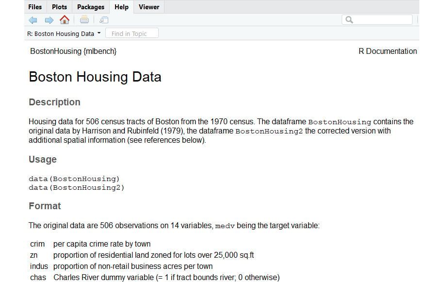
Figure 1.11: More information about the Boston Housing dataset
- The first n rows and last m rows in the data can be viewed as follows:
#Print the first 10 rows in the dataset
head(BostonHousing,10)
The output is as follows:
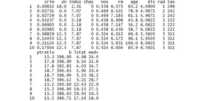
Figure 1.12: The first 10 rows of the Boston Housing dataset
- Print the last rows:
#Print the last rows in the dataset
tail(BostonHousing)
The output is as follows:
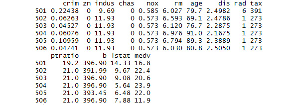
Figure 1.13: The last rows of the Boston Housing dataset
- Print the last 7 rows:
#Print the last 7 rows in the dataset
tail(BostonHousing,7)
The output is as follows:
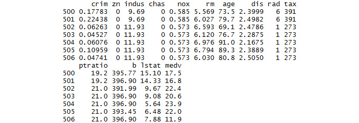
Figure 1.14: The last seven rows of the Boston Housing dataset
Thus, we have loaded a built-in dataset and read the first and last lines from the loaded dataset. We have also checked the total number of rows and columns in the dataset by cross-checking it with the information in the description provided.
Selectively running lines of code:
We can select lines of code within the script and click the Run option to run only those lines of code and not run the entire script:
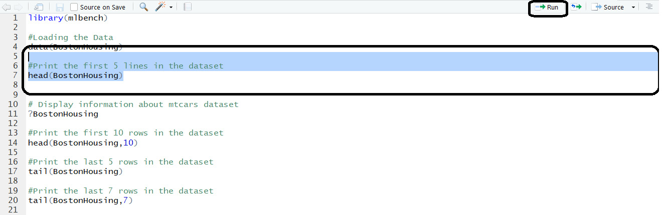
Figure 1.15: Selectively running the code
Now, we will move to viewing a summary of the data.
Exercise 4: Viewing Summaries of Data
To perform EDA, we need to know the data columns and data structure. In this exercise, we will cover the important functions that will help us explore data by finding the number of rows and columns in the data, the structure of the data, and the summary of the data.
- The columns names of the dataset can be viewed using the names() function:
# Display column names of GermanCredit
library(caret)
data(GermanCredit)
# Display column names of GermanCredit
names(GermanCredit)
A section of the output is as follows:
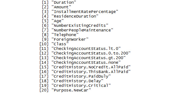
Figure 1.16: A section of names in the GermanCredit dataset
- The total number of rows in the data can be displayed using nrow:
# Display number of rows of GermanCredit
nrow(GermanCredit)
The output is as follows:
[1] 1000
- The total number of columns in the data can be displayed using ncol:
# Display number of columns of GermanCredit
ncol(GermanCredit)
The output is as follows:
[1] 62
- To know the structure of the data, use the str function:
# Display structure of GermanCredit
str(GermanCredit)
A section of the output is as follows:
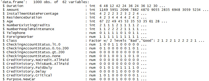
Figure 1.17: A section of names in the GermanCredit dataset
The column name Telephone is of numeric data type. Few data values are also displayed alongside it to explain the column values.
- The summary of the data can be obtained by the summary function:
# Display the summary of GermanCredit
summary(GermanCredit)
A section of the output is as follows:
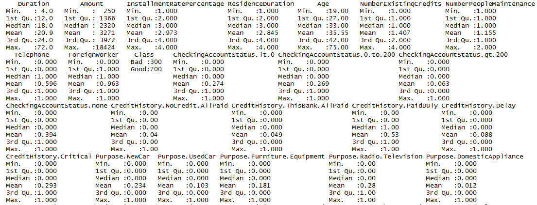
Figure 1.18: A section of the summary of the GermanCredit dataset
The summary provides information such as minimum value, 1st quantile, median, mean, 3rd quantile, and maximum value. The description of these values is as follows:
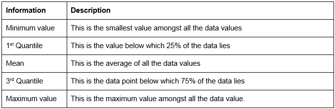
Figure 1.19: Summary parameters
- To view the summary of only one column, the particular column can be passed to the summary function:
# Display the summary of column 'Amount'
summary(GermanCredit$Amount)
The output is as follows:
Min. 1st Qu. Median Mean 3rd Qu. Max.
250 1366 2320 3271 3972 18424
We've had a glimpse of the data. Now, let's visualize it.
Visualizing the Data
Data can be difficult to interpret. In this section, we will interpret it using graphs and other visualizing tools.
Histograms: A histogram displays the total count for each value of the column. We can view a histogram using the hist() function in R. The function requires the column name to be passed as the first parameter and the color of the bars displayed on the histogram as the second parameter. The name of the x axis is automatically given by the function as the column name:
#Histogram for InstallmentRatePercentage column
hist(GermanCredit$InstallmentRatePercentage,col="red")
The output is as follows:
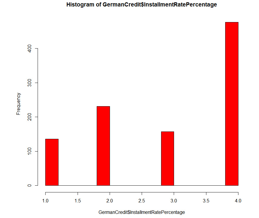
Figure 1.20: An example histogram
Bar plots: Bar plots in the ggplot package are another way to visualize the count for a column of data. The aes() function allows color coding of the values. In the upcoming example, the number of gears is plotted against the count. We have color-coded the gear values using the aes() function. Now, the factor() function is used to display only the unique values on the axis. For instance, the data contains 3, 4, and 5, and so you will see only these values on the x axis.
# Bar Plots
ggplot(GermanCredit, aes(factor(ResidenceDuration),fill= factor(ResidenceDuration))) +geom_bar()
The output is as follows:
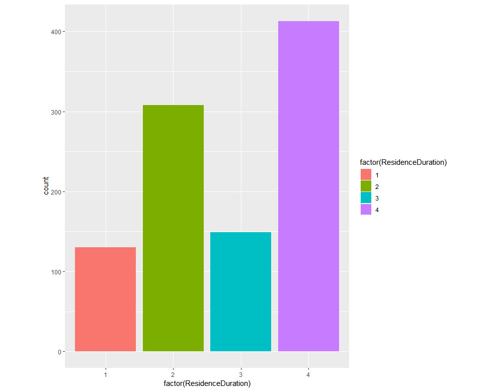
Figure 1.21: An example bar plot
Scatter plots: This requires ggplot, which we installed in the previous exercises. We plot Age on the x axis, Duration on the y axis, and Class in the form of color.
install.packages("ggplot2",dependencies = TRUE)
#Scatter Plot
library(ggplot2)
qplot(Age, Duration, data = GermanCredit, colour =factor(Class))
The output is as follows:
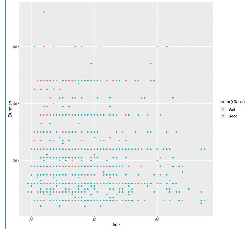
Figure 1.22: An example scatter plot
We can also view the third column by adding the facet parameter, as shown here:
#Scatter Plot
library(ggplot2)
qplot(Age,Duration,data=GermanCredit,facets=Class~.,colour=factor(Class))
The output is as follows:
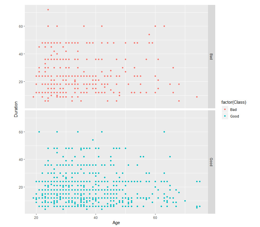
Figure 1.23: An example scatter plot facet
Box Plots: We can view data distribution using a box plot. It shows the minimum, maximum, 1st quartile, and 3rd quartile. In R, we can plot it using the boxplot() function. The dataframe is provided to the data parameter. NumberExistingCredits is the y axis and InstallmentRatePercentage is the x axis. The name of the plot can be provided in main. The names for the x axis and y axis are given in xlab and ylab, respectively. The color of the boxes can be set using the col parameter. An example is as follows:
# Boxplot of InstallmentRatePercentage by Car NumberExistingCredits
boxplot(InstallmentRatePercentage~NumberExistingCredits,
data=GermanCredit, main="Sample Box Plot",
xlab="InstallmentRatePercentage",
ylab="NumberExistingCredits",
col="red")
The output is as follows:
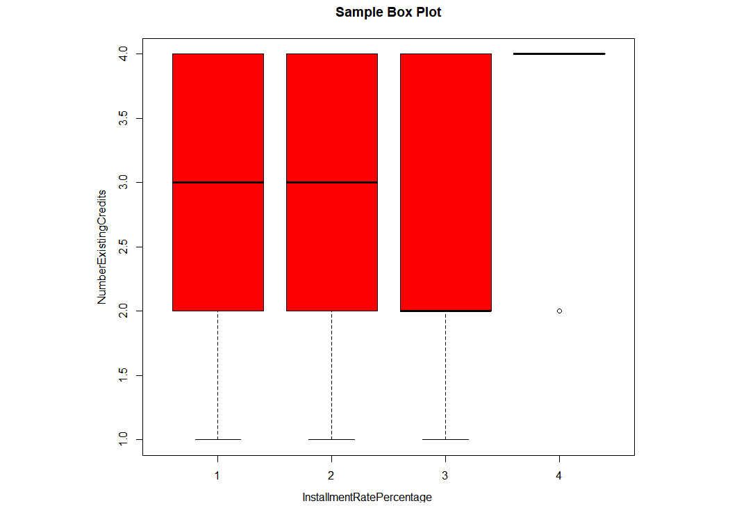
Figure 1.24: An example box plot
Correlation: The correlation plot is used to identify the correlation between two features. The correlation value can range from -1 to 1. Values between (0.5, 1) and (-0.5, -1) mean strong positive correlation and strong negative correlation, respectively. The corrplot() function can plot the correlation of all the features with each other in a simple map. It is also known as a correlation heatmap:
#Plot a correlation plot
GermanCredit_Subset=GermanCredit[,1:9]
install.packages("corrplot")
library(corrplot)
correlations = cor(GermanCredit_Subset)
print(correlations)
The output is as follows:
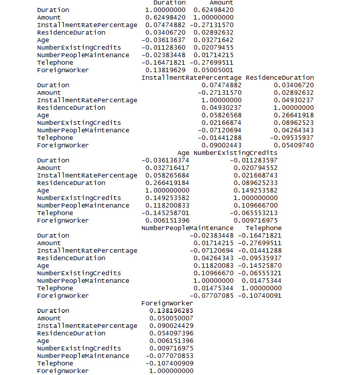
Figure 1.25: A section of the output for correlations
The plot for correlations is as follows:
corrplot(correlations, method="color")
The output is as follows:

Figure 1.26: A correlation plot
Density plot: The density plot can be used to view the distribution of the data. In this example, we are looking at the distribution of weight in the GermanCredit dataset:
#Density Plot
densityData <- density(GermanCredit$Duration)
plot(densityData, main="Kernel Density of Weight")
polygon(densityData, col="yellow", border="green")
The output is as follows:
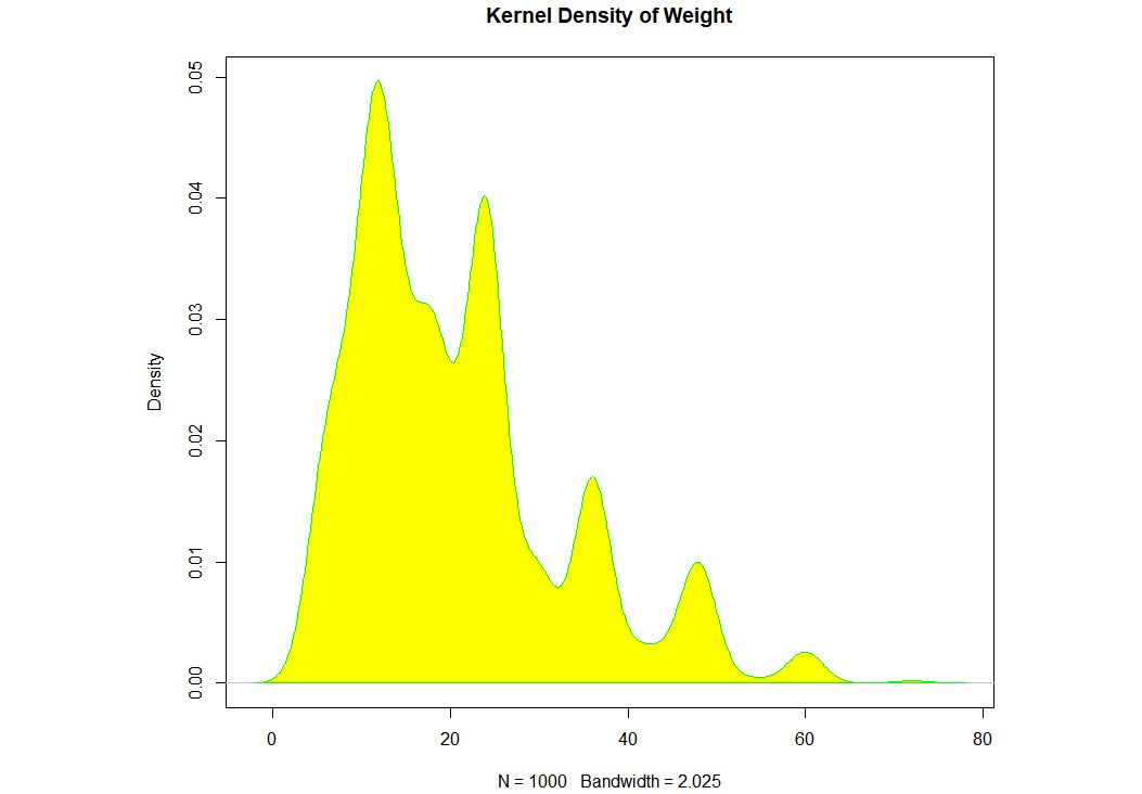
Figure 1.27: An example density plot
We have learned about different plots. It's time to use them with a dataset.
Activity 1: Finding the Distribution of Diabetic Patients in the PimaIndiansDiabetes Dataset
In this activity, we will load the PimaIndiansDiabetes dataset and find the age group of people with diabetes. The dataset can be found at https://github.com/TrainingByPackt/Practical-Machine-Learning-with-R/blob/master/Data/PimaIndiansDiabetes.csv.
The expected output should contain a bar plot of the count of positive and negative data present in the dataset with respect to age, as follows:
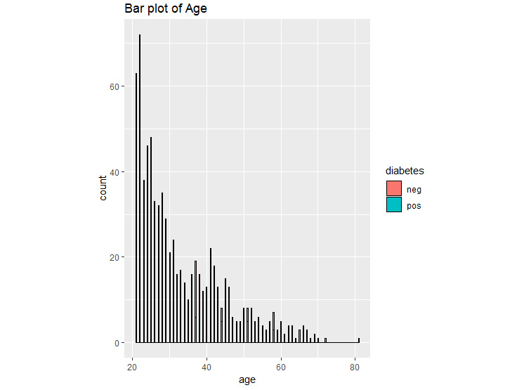
Figure 1.28: Bar plot for diabetes
These are the steps that will help you solve the activity:
- Load the dataset.
- Create a PimaIndiansDiabetesData variable for further use.
- View the first five rows using head().
- Display the different unique values for the diabetes column.
Note
The solution for this activity can be found on page 312.
Activity 2: Grouping the PimaIndiansDiabetes Data
During this activity, we will be viewing the summary of the PimaIndiansDiabetes dataset and grouping them to derive insights from the data.
These are the steps that will help you solve the activity:
- Print the structure of the dataset. [Hint: use str()]
- Print the summary of the dataset. [Hint: use summary()]
- Display the statistics of the dataset grouped by diabetes column. [Hint: use describeBy(data,groupby)]
The output will show the descriptive statistics of the value of diabetes grouped by the pregnant value.
#Descriptive statistics grouped by pregnant values
Descriptive statistics by group
group: neg
vars n mean sd median trimmed mad min max range skew kurtosis se
X1 1 500 68.18 18.06 70 69.97 11.86 0 122 122 -1.8 5.58 0.81
----------------------------------------------------------------------------------------------
group: pos
vars n mean sd median trimmed mad min max range skew kurtosis se
X1 1 268 70.82 21.49 74 73.99 11.86 0 114 114 -1.92 4.53 1.31
The output will show the descriptive statistics of the value of diabetes grouped by the pressure value.
#Descriptive statistics grouped by pressure values
Descriptive statistics by group
group: neg
vars n mean sd median trimmed mad min max range skew kurtosis se
X1 1 500 3.3 3.02 2 2.88 2.97 0 13 13 1.11 0.65 0.13
----------------------------------------------------------------------------------------------
group: pos
vars n mean sd median trimmed mad min max range skew kurtosis se
X1 1 268 4.87 3.74 4 4.6 4.45 0 17 17 0.5 -0.47 0.23
Note
The solution for this activity can be found on page 314.
Activity 3: Performing EDA on the PimaIndiansDiabetes Dataset
During this activity, we will be plotting the correlation among the fields in the PimaIndiansDiabetes dataset so that we can find which of the fields have a correlation with each other. Also, we will create a box plot to view the distribution of the data so that we know the range of the data, and which data points are outliers. The dataset can be found at https://github.com/TrainingByPackt/Practical-Machine-Learning-with-R/blob/master/Data/PimaIndiansDiabetes.csv.
These are the steps that will help you solve the activity:
- Load the PimaIndiansDiabetes dataset.
- View the correlation among the features of the PimaIndiansDiabetes dataset.
- Round it to the second nearest digit.
- Plot the correlation.
- Create a box plot to view the data distribution for the pregnant column and color by diabetes.
Once you complete the activity, you should obtain a boxplot of data distribution for the pregnant column, which is as follows:
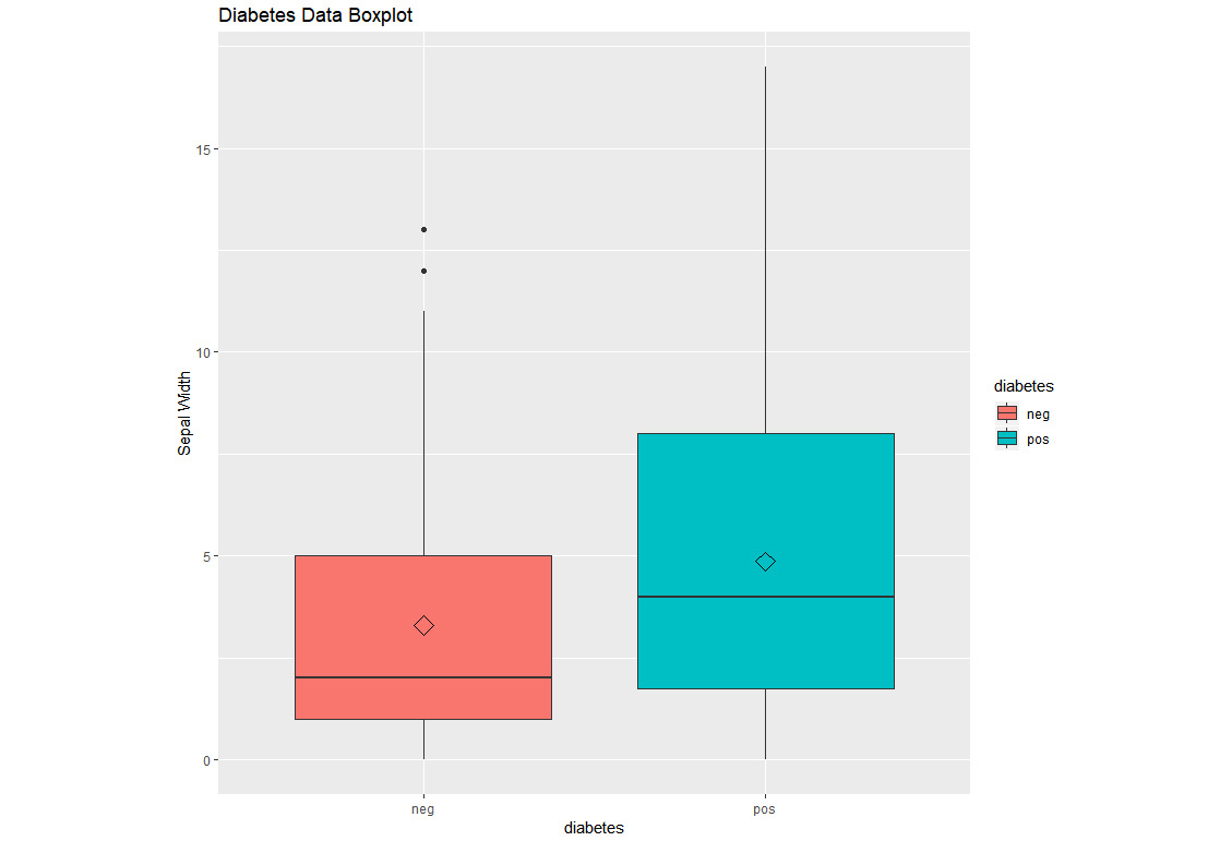
Figure 1.29: A box plot using ggplot
Note
The solution for this activity can be found on page 316.
We have learned how to perform correlation among all the columns in a dataset and how to plot a box plot for individual fields and then color it by certain categorical values.