
Regression
In this section, we will cover linear regression with single and multiple variables. Let's implement a linear regression model in R. We will predict the median value of an owner-occupied house in the Boston Housing dataset.
The Boston Housing dataset contains the following fields:
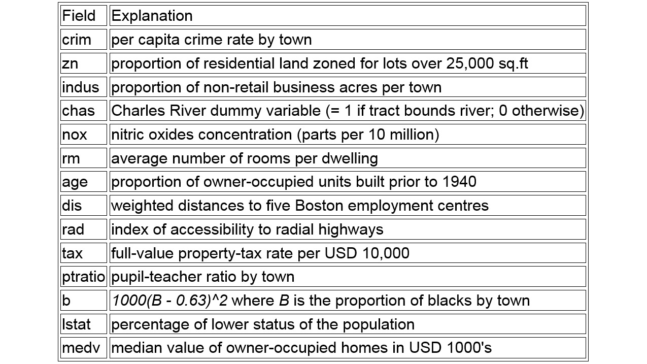
Figure 1.34: Boston Housing dataset fields
Here is a model for the indus field.
#Build a simple linear regression
model1 <- lm(medv~indus, data = BostonHousing)
#summary(model1)
AIC(model1)
The output is as follows:
[1] 3551.601
Build a model considering the age and dis fields:
model2 = lm(medv ~ age + dis, BostonHousing)
summary(model2)
AIC(model2)
Call:
lm(formula = medv ~ age + dis, data = BostonHousing)
Residuals:
Min 1Q Median 3Q Max
-15.661 -5.145 -1.900 2.173 31.114
Coefficients:
Estimate Std. Error t value Pr(>|t|)
(Intercept) 33.3982 2.2991 14.526 < 2e-16 ***
age -0.1409 0.0203 -6.941 1.2e-11 ***
dis -0.3170 0.2714 -1.168 0.243
---
Signif. codes: 0 ‘***’ 0.001 ‘**’ 0.01 ‘*’ 0.05 ‘.’ 0.1 ‘ ’ 1
Residual standard error: 8.524 on 503 degrees of freedom
Multiple R-squared: 0.1444, Adjusted R-squared: 0.141
F-statistic: 42.45 on 2 and 503 DF, p-value: < 2.2e-16
The output is as follows:
[1] 3609.558
AIC is the Akaike information criterion, denoting that the lower the value, the better the model performance. Therefore, the performance of model1 is superior to that of model2.
In a linear regression, it is important to find the distance between the actual output values and the predicted values. To calculate RMSE, we will find the square root of the mean of the squared error using sqrt(sum(error^2)/n).
We have learned to build various regression models with single or multiple fields in the preceding example.
Another type of supervised learning is classification. In the next exercise we will build a simple linear classifier, to see how similar that process is to the fitting of linear regression models. After that, you will dive into building more regression models in the activities.
Exercise 5: Building a Linear Classifier in R
In this exercise, we will build a linear classifier for the GermanCredit dataset using a linear discriminant analysis model.
The German Credit dataset contains the credit-worthiness of a customer (whether the customer is 'good' or 'bad' based on their credit history), account details, and so on. The dataset can be found at https://github.com/TrainingByPackt/Practical-Machine-Learning-with-R/blob/master/Data/GermanCredit.csv.
- Load the dataset:
# load the package
library(caret)
data(GermanCredit)
#OR
#GermanCredit <-read.csv("GermanCredit.csv")
- Subset the dataset:
#Subset the data
GermanCredit_Subset=GermanCredit[,1:10]
- Find the fit model:
# fit model
fit <- lda(Class~., data=GermanCredit_Subset)
- Summarize the fit:
# summarize the fit
summary(fit)
The output is as follows:
Length Class Mode
prior 2 -none- numeric
counts 2 -none- numeric
means 18 -none- numeric
scaling 9 -none- numeric
lev 2 -none- character
svd 1 -none- numeric
N 1 -none- numeric
call 3 -none- call
terms 3 terms call
xlevels 0 -none- list
- Make predictions.
# make predictions
predictions <- predict(fit, GermanCredit_Subset[,1:10],allow.new.levels=TRUE)$class
- Calculate the accuracy of the model:
# summarize accuracy
accuracy <- mean(predictions == GermanCredit_Subset$Class)
- Print accuracy:
accuracy
The output is as follows:
[1] 0.71
In this exercise, we have trained a linear classifier to predict the credit rating of customers with an accuracy of 71%. In chapter 4, Introduction to neuralnet and Evaluation Methods, we will try to beat that accuracy, and investigate whether 71% is actually a good accuracy for the given dataset.
Activity 4: Building Linear Models for the GermanCredit Dataset
In this activity, we will implement a linear regression model on the GermanCredit dataset. The dataset can be found at https://github.com/TrainingByPackt/Practical-Machine-Learning-with-R/blob/master/Data/GermanCredit.csv.
These are the steps that will help you solve the activity:
- Load the dataset.
- Subset the data.
- Fit a linear model for predicting Duration using lm().
- Summarize the results.
- Use predict() to predict the output variable in the subset.
- Calculate Root Mean Squared Error.
Expected output: In this activity, we expect an RMSE value of 76.3849.
Note
The solution for this activity can be found on page 319.
In this activity, we have learned to build a linear model, make predictions on new data, and evaluate performance using RMSE.
Activity 5: Using Multiple Variables for a Regression Model for the Boston Housing Dataset
In this activity, we will build a regression model and explore multiple variables from the dataset.
Refer to the example of linear regression performed with one variable and use multiple variables in this activity.
The dataset can be found at https://github.com/TrainingByPackt/Practical-Machine-Learning-with-R/blob/master/Data/BostonHousing.csv.
These are the steps that will help you solve the activity:
- Load the dataset.
- Build a regression model using multiple variables.
- View the summary of the built regression model.
- Plot the regression model using the plot() function.
The final graph for the regression model will look as follows:
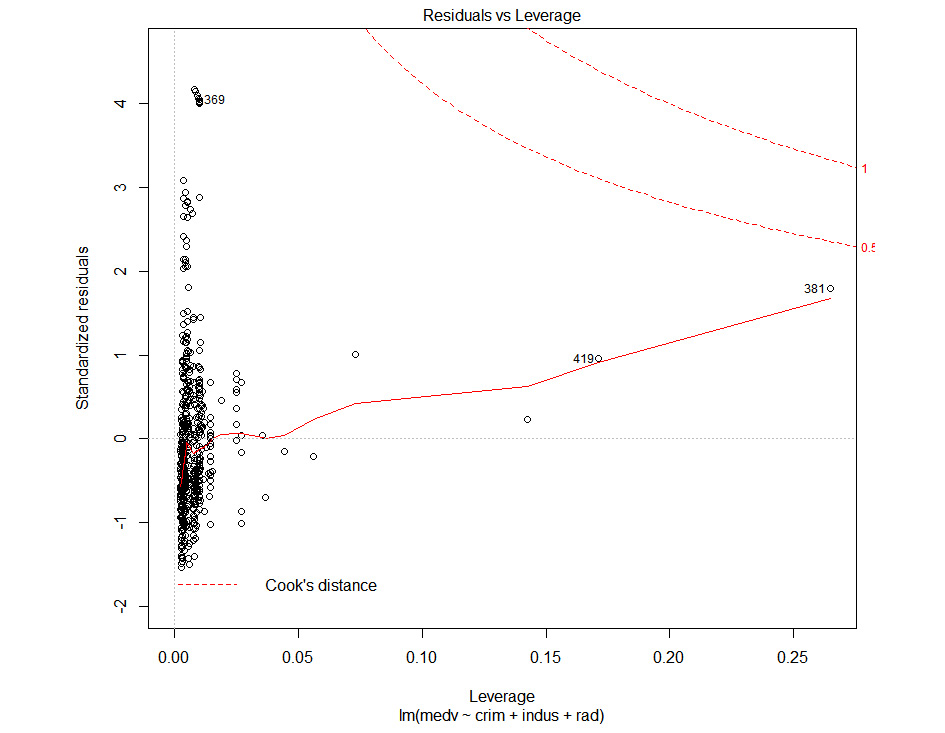
Figure 1.35: Cook's distance plot
Note
The solution for this activity can be found on page 320.
We have now explored the datasets with one or more variables.