

Data Representation
The main objective of machine learning is to build models that understand data and find underlying patterns. In order to do so, it is very important to feed the data in a way that is interpretable by the computer. To feed the data into a model, it must be represented as a table or a matrix of the required dimensions. Converting your data into the correct tabular form is one of the first steps before pre-processing can properly begin.
Data Represented in a Table
Data should be arranged in a two-dimensional space made up of rows and columns. This type of data structure makes it easy to understand the data and pinpoint any problems. An example of some raw data stored as a CSV (comma separated values) file is shown here:

Figure 1.1: Raw data in CSV format
The representation of the same data in a table is as follows:
Figure 1.2: CSV data in table format
If you compare the data in CSV and table formats, you will see that there are missing values in both. We will cover what to do with these later in the chapter. To load a CSV file and work on it as a table, we use the pandas library. The data here is loaded into tables called DataFrames.
Note
To learn more about pandas, visit the following link: http://pandas.pydata.org/pandas-docs/version/0.15/tutorials.html.
Independent and Target Variables
The DataFrame that we use contains variables or features that can be classified into two categories. These are independent variables (also called predictor variables) and dependent variables (also called target variables). Independent variables are used to predict the target variable. As the name suggests, independent variables should be independent of each other. If they are not, this will need to be addressed in the pre-processing (cleaning) stage.
Independent Variables
These are all the features in the DataFrame except the target variable. They are of size (m, n), where m is the number of observations and n is the number of features. These variables must be normally distributed and should NOT contain:
- Missing or NULL values
- Highly categorical data features or high cardinality (these terms will be covered in more detail later)
- Outliers
- Data on different scales
- Human error
- Multicollinearity (independent variables that are correlated)
- Very large independent feature sets (too many independent variables to be manageable)
- Sparse data
- Special characters
Feature Matrix and Target Vector
A single piece of data is called a scalar. A group of scalars is called a vector, and a group of vectors is called a matrix. A matrix is represented in rows and columns. Feature matrix data is made up of independent columns, and the target vector depends on the feature matrix columns. To get a better understanding of this, let's look at the following table:
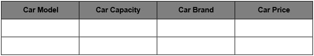
Figure 1.3: Table containing car details
As you can see in the table, there are various columns: Car Model, Car Capacity, Car Brand, and Car Price. All columns except Car Price are independent variables and represent the feature matrix. Car Price is the dependent variable that depends on the other columns (Car Model, Car Capacity, and Car Brand). It is a target vector because it depends on the feature matrix data. In the next section, we'll go through an exercise based on features and a target matrix to get a thorough understanding.
Note
All exercises and activities will be primarily developed in Jupyter Notebook. It is recommended to keep a separate notebook for different assignments unless advised not to. Also, to load a sample dataset, the pandas library will be used, because it displays the data as a table. Other ways to load data will be explained in further sections.
Exercise 1: Loading a Sample Dataset and Creating the Feature Matrix and Target Matrix
In this exercise, we will be loading the House_price_prediction dataset into the pandas DataFrame and creating feature and target matrices. The House_price_prediction dataset is taken from the UCI Machine Learning Repository. The data was collected from various suburbs of the USA and consists of 5,000 entries and 6 features related to houses. Follow these steps to complete this exercise:
Note
The House_price_prediction dataset can be found at this location: https://github.com/TrainingByPackt/Data-Science-with-Python/blob/master/Chapter01/Data/USA_Housing.csv.
- Open a Jupyter notebook and add the following code to import pandas:
import pandas as pd
- Now we need to load the dataset into a pandas DataFrame. As the dataset is a CSV file, we'll be using the read_csv() function to read the data. Add the following code to do this:
dataset = "https://github.com/TrainingByPackt/Data-Science-with-Python/blob/master/Chapter01/Data/USA_Housing.csv"
df = pd.read_csv(dataset, header = 0)
As you can see in the preceding code, the data is stored in a variable named df.
- To print all the column names of the DataFrame, we'll use the df.columns command. Write the following code in the notebook:
df.columns
The preceding code generates the following output:
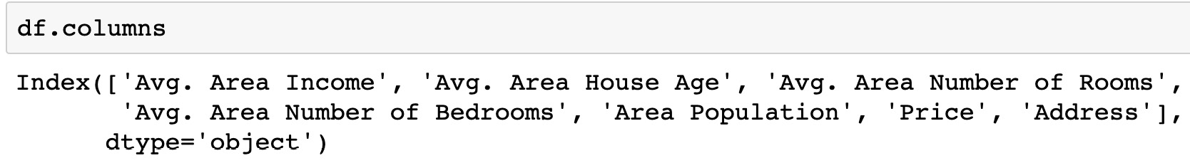
Figure 1.4: List of columns present in the dataframe
- The dataset contains n number of data points. We can find the total number of rows using the following command:
df.index
The preceding code generates the following output:

Figure 1.5: Total Index in the dataframe
As you can see in the preceding figure, our dataset contains 5000 rows, from index 0 to 5000.
Note
You can use the set_index() function in pandas to convert a column into an index of rows in a DataFrame. This is a bit like using the values in that column as your row labels.
Dataframe.set_index('column name', inplace = True')'
- Let's set the Address column as an index and reset it back to the original DataFrame. The pandas library provides the set_index() method to convert a column into an index of rows in a DataFrame. Add the following code to implement this:
df.set_index('Address', inplace=True)
df
The preceding code generates the following output:
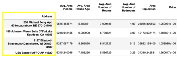
Figure 1.6: DataFrame with an indexed Address column
The inplace parameter in the set_index() function is by default set to False. If the value is changed to True, then whatever operation we perform the content of the DataFrame changes directly without the copy being created.
- In order to reset the index of the given object, we use the reset_index() function. Write the following code to implement this:
df.reset_index(inplace=True)
df
The preceding code generates the following output:
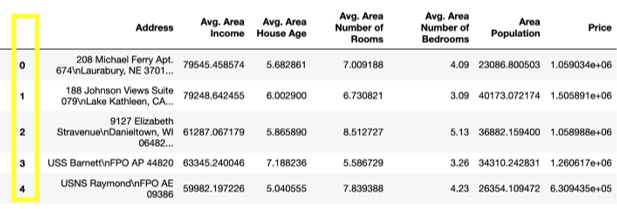
Figure 1.7: DataFrame with the index reset
Note
The index is like a name given to a row and column. Rows and columns both have an index. You can index by row/column number or row/column name.
- We can retrieve the first four rows and the first three columns using a row number and column number. This can be done using the iloc indexer in pandas, which retrieves data using index positions. Add the following code to do this:
df.iloc[0:4 , 0:3]
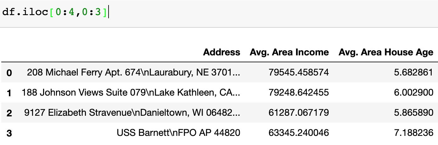
Figure 1.8: Dataset of four rows and three columns
- To retrieve the data using labels, we use the loc indexer. Add the following code to retrieve the first five rows of the Income and Age columns:
df.loc[0:4 , ["Avg. Area Income", "Avg. Area House Age"]]

Figure 1.9: Dataset of five rows and two columns
- Now create a variable called X to store the independent features. In our dataset, we will consider all features except Price as independent variables, and we will use the drop() function to include them. Once this is done, we print out the top five instances of the X variable. Add the following code to do this:
X = df.drop('Price', axis=1)
X.head()
The preceding code generates the following output:
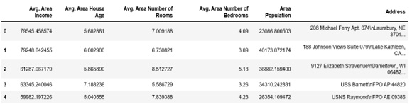
Figure 1.10: Dataset showing the first five rows of the feature matrix
Note
The default number of instances that will be taken for the head is five, so if you don't specify the number then it will by default output five observations. The axis parameter in the preceding screenshot denotes whether you want to drop the label from rows (axis = 0) or columns (axis = 1).
- Print the shape of your newly created feature matrix using the X.shape command. Add the following code to do this:
X.shape
The preceding code generates the following output:

Figure 1.11: Shape of the feature matrix
In the preceding figure, the first value indicates the number of observations in the dataset (5000), and the second value represents the number of features (6).
- Similarly, we will create a variable called y that will store the target values. We will use indexing to grab the target column. Indexing allows you to access a section of a larger element. In this case, we want to grab the column named Price from the df DataFrame. Then, we want to print out the top 10 values of the variable. Add the following code to implement this:
y = df['Price']
y.head(10)
The preceding code generates the following output:
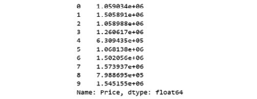
Figure 1.12: Dataset showing the first 10 rows of the target matrix
- Print the shape of your new variable using the y.shape command. The shape should be one-dimensional, with a length equal to the number of observations (5000) only. Add the following code to implement this:
y.shape
The preceding code generates the following output:

Figure 1.13: Shape of the target matrix
You have successfully created the feature and target matrices of a dataset. You have completed the first step in the process of building a predictive model. This model will learn the patterns from the feature matrix (columns in X) and how they map to the values in the target vector (y). These patterns can then be used to predict house prices from new data based on the features of those new houses.
In the next section, we will explore more steps involved in pre-processing.