

Data Transformation
Previously, we saw how we can combine data from different sources into a unified dataframe. Now, we have a lot of columns that have different types of data. Our goal is to transform the data into a machine-learning-digestible format. All machine learning algorithms are based on mathematics. So, we need to convert all the columns into numerical format. Before that, let's see all the different types of data we have.
Taking a broader perspective, data is classified into numerical and categorical data:
- Numerical: As the name suggests, this is numeric data that is quantifiable.
- Categorical: The data is a string or non-numeric data that is qualitative in nature.
Numerical data is further divided into the following:
- Discrete: To explain in simple terms, any numerical data that is countable is called discrete, for example, the number of people in a family or the number of students in a class. Discrete data can only take certain values (such as 1, 2, 3, 4, etc).
- Continuous: Any numerical data that is measurable is called continuous, for example, the height of a person or the time taken to reach a destination. Continuous data can take virtually any value (for example, 1.25, 3.8888, and 77.1276).
Categorical data is further divided into the following:
- Ordered: Any categorical data that has some order associated with it is called ordered categorical data, for example, movie ratings (excellent, good, bad, worst) and feedback (happy, not bad, bad). You can think of ordered data as being something you could mark on a scale.
- Nominal: Any categorical data that has no order is called nominal categorical data. Examples include gender and country.
From these different types of data, we will focus on categorical data. In the next section, we'll discuss how to handle categorical data.
Handling Categorical Data
There are some algorithms that can work well with categorical data, such as decision trees. But most machine learning algorithms cannot operate directly with categorical data. These algorithms require the input and output both to be in numerical form. If the output to be predicted is categorical, then after prediction we convert them back to categorical data from numerical data. Let's discuss some key challenges that we face while dealing with categorical data:
- High cardinality: Cardinality means uniqueness in data. The data column, in this case, will have a lot of different values. A good example is User ID – in a table of 500 different users, the User ID column would have 500 unique values.
- Rare occurrences: These data columns might have variables that occur very rarely and therefore would not be significant enough to have an impact on the model.
- Frequent occurrences: There might be a category in the data columns that occurs many times with very low variance, which would fail to make an impact on the model.
- Won't fit: This categorical data, left unprocessed, won't fit our model.
Encoding
To address the problems associated with categorical data, we can use encoding. This is the process by which we convert a categorical variable into a numerical form. Here, we will look at three simple methods of encoding categorical data.
Replacing
This is a technique in which we replace the categorical data with a number. This is a simple replacement and does not involve much logical processing. Let's look at an exercise to get a better idea of this.
Exercise 6: Simple Replacement of Categorical Data with a Number
In this exercise, we will use the student dataset that we saw earlier. We will load the data into a pandas dataframe and simply replace all the categorical data with numbers. Follow these steps to complete this exercise:
Note
The student dataset can be found at this location: https://github.com/TrainingByPackt/Data-Science-with-Python/blob/master/Chapter01/Data/student.csv.
- Open a Jupyter notebook and add a new cell. Write the following code to import pandas and then load the dataset into the pandas dataframe:
import pandas as pd
import numpy as np
dataset = "https://github.com/TrainingByPackt/Data-Science-with-Python/blob/master/Chapter01/Data/student.csv"
df = pd.read_csv(dataset, header = 0)
- Find the categorical column and separate it out with a different dataframe. To do so, use the select_dtypes() function from pandas:
df_categorical = df.select_dtypes(exclude=[np.number])
df_categorical
The preceding code generates the following output:

Figure 1.28: Categorical columns of the dataframe
- Find the distinct unique values in the Grade column. To do so, use the unique() function from pandas with the column name:
df_categorical['Grade'].unique()
The preceding code generates the following output:

Figure 1.29: Unique values in the Grade column
- Find the frequency distribution of each categorical column. To do so, use the value_counts() function on each column. This function returns the counts of unique values in an object:
df_categorical.Grade.value_counts()
The output of this step is as follows:

Figure 1.30: Total count of each unique value in the Grade column
- For the Gender column, write the following code:
df_categorical.Gender.value_counts()
The output of this code is as follows:

Figure 1.31: Total count of each unique value in the Gender column
- Similarly, for the Employed column, write the following code:
df_categorical.Employed.value_counts()
The output of this code is as follows:

Figure 1.32: Total count of each unique value in the Employed column
- Replace the entries in the Grade column. Replace 1st class with 1, 2nd class with 2, and 3rd class with 3. To do so, use the replace() function:
df_categorical.Grade.replace({"1st Class":1, "2nd Class":2, "3rd Class":3}, inplace= True)
- Replace the entries in the Gender column. Replace Male with 0 and Female with 1. To do so, use the replace() function:
df_categorical.Gender.replace({"Male":0,"Female":1}, inplace= True)
- Replace the entries in the Employed column. Replace no with 0 and yes with 1. To do so, use the replace() function:
df_categorical.Employed.replace({"yes":1,"no":0}, inplace = True)
- Once all the replacements for three columns are done, we need to print the dataframe. Add the following code:
df_categorical.head()

Figure 1.33: Numerical data after replacement
You have successfully converted the categorical data to numerical data using a simple manual replacement method. We will now move on to look at another method of encoding categorical data.
Label Encoding
This is a technique in which we replace each value in a categorical column with numbers from 0 to N-1. For example, say we've got a list of employee names in a column. After performing label encoding, each employee name will be assigned a numeric label. But this might not be suitable for all cases because the model might consider numeric values to be weights assigned to the data. Label encoding is the best method to use for ordinal data. The scikit-learn library provides LabelEncoder(), which helps with label encoding. Let's look at an exercise in the next section.
Exercise 7: Converting Categorical Data to Numerical Data Using Label Encoding
In this exercise, we will load the Banking_Marketing.csv dataset into a pandas dataframe and convert categorical data to numeric data using label encoding. Follow these steps to complete this exercise:
Note
The Banking_Marketing.csv dataset can be found here: https://github.com/TrainingByPackt/Master-Data-Science-with-Python/blob/master/Chapter%201/Data/Banking_Marketing.csv.
- Open a Jupyter notebook and add a new cell. Write the code to import pandas and load the dataset into the pandas dataframe:
import pandas as pd
import numpy as np
dataset = 'https://github.com/TrainingByPackt/Master-Data-Science-with-Python/blob/master/Chapter%201/Data/Banking_Marketing.csv'
df = pd.read_csv(dataset, header=0)
- Before doing the encoding, remove all the missing data. To do so, use the dropna() function:
df = df.dropna()
- Select all the columns that are not numeric using the following code:
data_column_category = df.select_dtypes(exclude=[np.number]).columns
data_column_category
To understand how the selection looks, refer to the following screenshot:

Figure 1.34: Non-numeric columns of the dataframe
- Print the first five rows of the new dataframe. Add the following code to do this:
df[data_column_category].head()
The preceding code generates the following output:
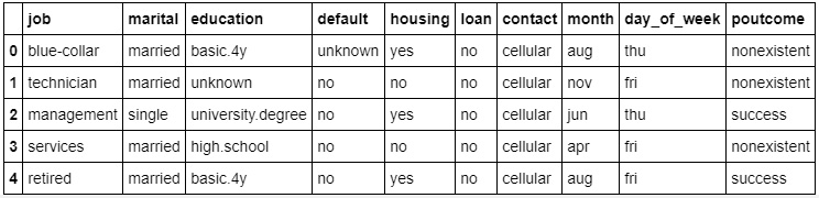
Figure 1.35: Non-numeric values for the columns
- Iterate through this category column and convert it to numeric data using LabelEncoder(). To do so, import the sklearn.preprocessing package and use the LabelEncoder() class to transform the data:
#import the LabelEncoder class
from sklearn.preprocessing import LabelEncoder
#Creating the object instance
label_encoder = LabelEncoder()
for i in data_column_category:
df[i] = label_encoder.fit_transform(df[i])
print("Label Encoded Data: ")
df.head()
The preceding code generates the following output:
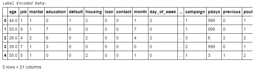
Figure 1.36: Values of non-numeric columns converted into numeric form
In the preceding screenshot, we can see that all the values have been converted from categorical to numerical. Here, the original values have been transformed and replaced with the newly encoded data.
You have successfully converted categorical data to numerical data using the LabelEncoder method. In the next section, we'll explore another type of encoding: one-hot encoding.
One-Hot Encoding
In label encoding, categorical data is converted to numerical data, and the values are assigned labels (such as 1, 2, and 3). Predictive models that use this numerical data for analysis might sometimes mistake these labels for some kind of order (for example, a model might think that a label of 3 is "better" than a label of 1, which is incorrect). In order to avoid this confusion, we can use one-hot encoding. Here, the label-encoded data is further divided into n number of columns. Here, n denotes the total number of unique labels generated while performing label encoding. For example, say that three new labels are generated through label encoding. Then, while performing one-hot encoding, the columns will be divided into three parts. So, the value of n is 3. Let's look at an exercise to get further clarification.
Exercise 8: Converting Categorical Data to Numerical Data Using One-Hot Encoding
In this exercise, we will load the Banking_Marketing.csv dataset into a pandas dataframe and convert the categorical data into numeric data using one-hot encoding. Follow these steps to complete this exercise:
Note
The Banking_Marketing dataset can be found here: https://github.com/TrainingByPackt/Data-Science-with-Python/blob/master/Chapter01/Data/Banking_Marketing.csv.
- Open a Jupyter notebook and add a new cell. Write the code to import pandas and load the dataset into a pandas dataframe:
import pandas as pd
import numpy as np
from sklearn.preprocessing import OneHotEncoder
dataset = 'https://github.com/TrainingByPackt/Master-Data-Science-with-Python/blob/master/Chapter%201/Data/Banking_Marketing.csv'
#reading the data into the dataframe into the object data
df = pd.read_csv(dataset, header=0)
- Before doing the encoding, remove all the missing data. To do so, use the dropna() function:
df = df.dropna()
- Select all the columns that are not numeric using the following code:
data_column_category = df.select_dtypes(exclude=[np.number]).columns
data_column_category
The preceding code generates the following output:

Figure 1.37: Non-numeric columns of the dataframe
- Print the first five rows of the new dataframe. Add the following code to do this:
df[data_column_category].head()
The preceding code generates the following output:
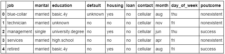
Figure 1.38: Non-numeric values for the columns
- Iterate through these category columns and convert them to numeric data using OneHotEncoder. To do so, import the sklearn.preprocessing package and avail yourself of the OneHotEncoder() class do the transformation. Before performing one-hot encoding, we need to perform label encoding:
#performing label encoding
from sklearn.preprocessing import LabelEncoder
label_encoder = LabelEncoder()
for i in data_column_category:
df[i] = label_encoder.fit_transform(df[i])
print("Label Encoded Data: ")
df.head()
The preceding code generates the following output:

Figure 1.39: Values of non-numeric columns converted into numeric data
- Once we have performed label encoding, we execute one-hot encoding. Add the following code to implement this:
#Performing Onehot Encoding
onehot_encoder = OneHotEncoder(sparse=False)
onehot_encoded = onehot_encoder.fit_transform(df[data_column_category])
- Now we create a new dataframe with the encoded data and print the first five rows. Add the following code to do this:
#Creating a dataframe with encoded data with new column name
onehot_encoded_frame = pd.DataFrame(onehot_encoded, columns = onehot_encoder.get_feature_names(data_column_category))
onehot_encoded_frame.head()
The preceding code generates the following output:
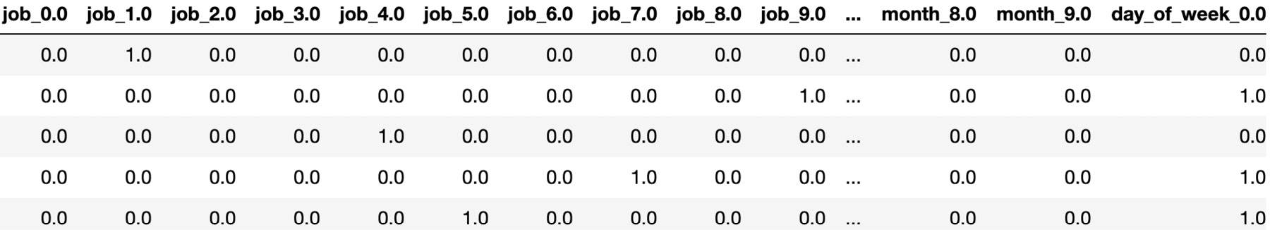
Figure 1.40: Columns with one-hot encoded values
- Due to one-hot encoding, the number of columns in the new dataframe has increased. In order to view and print all the columns created, use the columns attribute:
onehot_encoded_frame.columns
The preceding code generates the following output:

Figure 1.41: List of new columns generated after one-hot encoding
- For every level or category, a new column is created. In order to prefix the category name with the column name you can use this alternate way to create one-hot encoding. In order to prefix the category name with the column name, write the following code:
df_onehot_getdummies = pd.get_dummies(df[data_column_category], prefix=data_column_category)
data_onehot_encoded_data = pd.concat([df_onehot_getdummies,df[data_column_number]],axis = 1)
data_onehot_encoded_data.columns
The preceding code generates the following output:
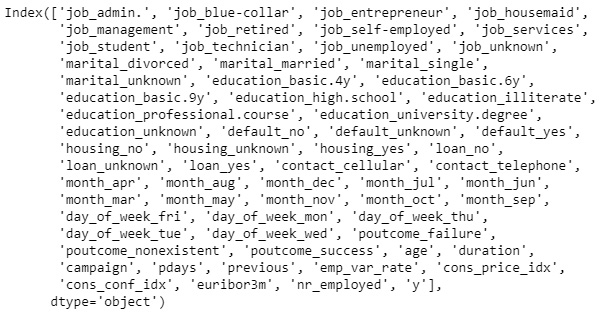
Figure 1.42: List of new columns containing the categories
You have successfully converted categorical data to numerical data using the OneHotEncoder method.
We will now move onto another data preprocessing step – how to deal with a range of magnitudes in your data.