
Data in Different Scales
In real life, values in a dataset might have a variety of different magnitudes, ranges, or scales. Algorithms that use distance as a parameter may not weigh all these in the same way. There are various data transformation techniques that are used to transform the features of our data so that they use the same scale, magnitude, or range. This ensures that each feature has an appropriate effect on a model's predictions.
Some features in our data might have high-magnitude values (for example, annual salary), while others might have relatively low values (for example, the number of years worked at a company). Just because some data has smaller values does not mean it is less significant. So, to make sure our prediction does not vary because of different magnitudes of features in our data, we can perform feature scaling, standardization, or normalization (these are three similar ways of dealing with magnitude issues in data).
Exercise 9: Implementing Scaling Using the Standard Scaler Method
In this exercise, we will load the Wholesale customer's data.csv dataset into the pandas dataframe and perform scaling using the standard scaler method. This dataset refers to clients of a wholesale distributor. It includes the annual spending in monetary units on diverse product categories. Follow these steps to complete this exercise:
Note
The Wholesale customer dataset can be found here: https://github.com/TrainingByPackt/Data-Science-with-Python/blob/master/Chapter01/Data/Wholesale%20customers%20data.csv.
- Open a Jupyter notebook and add a new cell. Write the code to import pandas and load the dataset into the pandas dataframe:
import pandas as pd
dataset = 'https://github.com/TrainingByPackt/Data-Science-with-Python/blob/master/Chapter01/Data/Wholesale%20customers%20data.csv'
df = pd.read_csv(dataset, header=0)
- Check whether there is any missing data. If there is, drop the missing data:
null_ = df.isna().any()
dtypes = df.dtypes
info = pd.concat([null_,dtypes],axis = 1,keys = ['Null','type'])
print(info)
The preceding code generates the following output:

Figure 1.43: Different columns of the dataframe
As we can see, there are eight columns present in the dataframe, all of type int64. Since the null value is False, it means there are no null values present in any of the columns. Thus, there is no need to use the dropna() function.
- Now perform standard scaling and print the first five rows of the new dataset. To do so, use the StandardScaler() class from sklearn.preprocessing and implement the fit_transorm() method:
from sklearn import preprocessing
std_scale = preprocessing.StandardScaler().fit_transform(df)
scaled_frame = pd.DataFrame(std_scale, columns=df.columns)
scaled_frame.head()
The preceding code generates the following output:
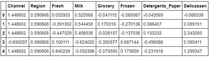
Figure 1.44: Data of the features scaled into a uniform unit
Using the StandardScaler method, we have scaled the data into a uniform unit over all the columns. As you can see in the preceding table, the values of all the features have been converted into a uniform range of the same scale. Because of this, it becomes easier for the model to make predictions.
You have successfully scaled the data using the StandardScaler method. In the next section, we'll have a go at an exercise in which we'll implement scaling using the MinMax scaler method.
Exercise 10: Implementing Scaling Using the MinMax Scaler Method
In this exercise, we will be loading the Wholesale customers data.csv dataset into a pandas dataframe and perform scaling using the MinMax scaler method. Follow these steps to complete this exercise:
Note
The Whole customers data.csv dataset can be found here: https://github.com/TrainingByPackt/Data-Science-with-Python/blob/master/Chapter01/Data/Wholesale%20customers%20data.csv.
- Open a Jupyter notebook and add a new cell. Write the following code to import the pandas library and load the dataset into a pandas dataframe:
import pandas as pd
dataset = 'https://github.com/TrainingByPackt/Data-Science-with-Python/blob/master/Chapter01/Data/Wholesale%20customers%20data.csv'
df = pd.read_csv(dataset, header=0)
- Check whether there is any missing data. If there is, drop the missing data:
null_ = df.isna().any()
dtypes = df.dtypes
info = pd.concat([null_,dtypes],axis = 1,keys = ['Null','type'])
print(info)
The preceding code generates the following output:
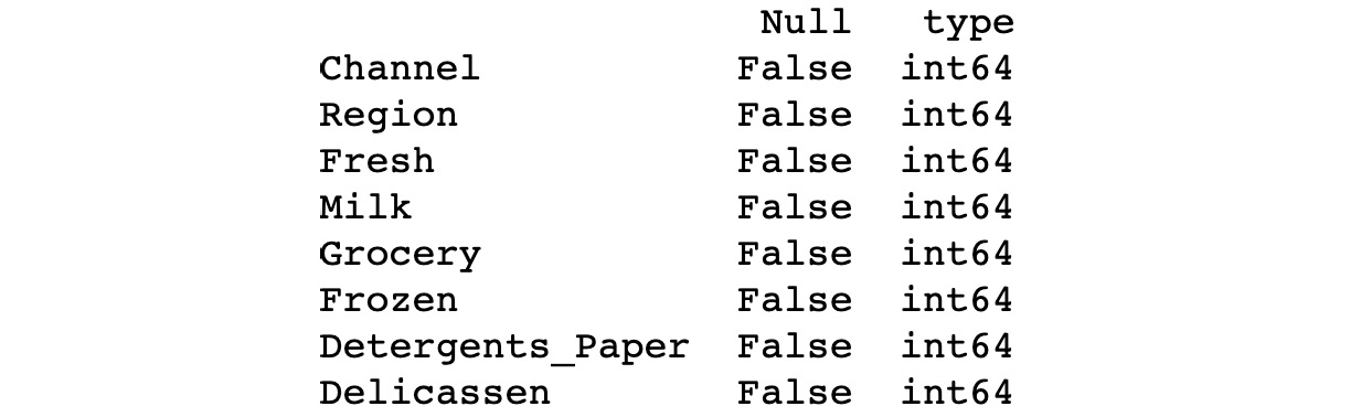
Figure 1.45: Different columns of the dataframe
As we can see, there are eight columns present in the dataframe, all of type int64. Since the null value is False, it means there are no null values present in any of the columns. Thus, there is no need to use the dropna() function.
- Perform MinMax scaling and print the initial five values of the new dataset. To do so, use the MinMaxScaler() class from sklearn.preprocessing and implement the fit_transorm() method. Add the following code to implement this:
from sklearn import preprocessing
minmax_scale = preprocessing.MinMaxScaler().fit_transform(df)
scaled_frame = pd.DataFrame(minmax_scale,columns=df.columns)
scaled_frame.head()
The preceding code generates the following output:
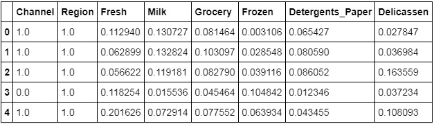
Figure 1.46: Data of the features scaled into a uniform unit
Using the MinMaxScaler method, we have again scaled the data into a uniform unit over all the columns. As you can see in the preceding table, the values of all the features have been converted into a uniform range of the same scale. You have successfully scaled the data using the MinMaxScaler method.
In the next section, we'll explore another pre-processing task: data discretization.