
We build models so that we can learn something about the data we are training on and about the relationships between the features of the dataset. This learning can inform us when we encounter new observations. However, we must realize that the observations we interact with in the real world and the format of data needed to train machine learning models are very different. Working with text data is a prime example of this. When we read text, we are able to understand each word and apply context given each word in relation to the surrounding words -- not a trivial task.However, machines are unable to interpret this contextual information. Unless it specifically encoded, they have no idea how to convert text into something that can be an input numerical. Therefore, we must represent the data appropriately, often by converting non-numerical data types, for example, converting text, dates, and categorical variables into numerical ones.
Much of the data fed into machine learning problems is two-dimensional, and can be represented as rows or columns. Images are a good example of a dataset that may be three-or even four-dimensional. The shape of each image will be two-dimensional (a height and a width), the number of images together will add a third dimension, and a color channel (red, green, blue) will add a fourth.

Figure 1.3: A color image and its representation as red, green, and blue images
Note
We have used datasets from this repository: Dua, D. and Graff, C. (2019). UCI Machine Learning Repository [http://archive.ics.uci.edu/ml]. Irvine, CA: University of California, School of Information and Computer Science.
The following figure shows a few rows from a marketing dataset taken from the UCI repository. The dataset presents marketing campaign results of a Portuguese banking institution. The columns of the table show various details about each customer, while the final column, y, shows whether or not the customer subscribed to the product that was featured in the marketing campaign.
One objective of analyzing the dataset could be to try and use the information given to predict whether a given customer subscribed to the product (that is, to try and predict what is in column y for each row). We can then check whether we were correct by comparing our predictions to column y. The longer-term benefit of this is that we could then use our model to predict whether new customers will subscribe to the product, or whether existing customers will subscribe to another product after a different campaign.

Figure 1.4: An image showing the first 20 instances of the marketing dataset
Data can be in different forms and can be available in many places. Datasets for beginners are often given in a flat format, which means that they are two-dimensional, with rows and columns. Other common forms of data may include images, JSON objects, and text documents. Each type of data format has to be loaded in specific ways. For example, numerical data can be loaded into memory using the NumPy library, which is an efficient library for working with matrices in Python. However, we would not be able to load our marketing data .csv into memory using the NumPy library because the dataset contains string values. For our dataset, we will use the pandas library becauseof its ability to easily work with various data types, such as strings, integers, floats, and binary values. In fact, pandas is dependent on NumPy for operations on numerical data types. pandas is also able to read JSON, Excel documents, and databases using SQL queries, which makes the library common amongst practitioners for loading and manipulating data in Python.
Here is an example of how to load a CSV file using the NumPy library. We use the skiprows argument in case is there is a header, which usually contains column names:
import numpy as np
data = np.loadtxt(filename, delimiter=",", skiprows=1)
Here's an example of loading data using the pandas library:
import pandas as pd
data = pd.read_csv(filename, delimiter=",")
Here we are loading in a CSV file. The default delimiter is a comma, and so passing this as an argument is not necessary, but is useful to see. The pandas library can also handle non-numeric datatypes, which makes the library more flexible:
import pandas as pd
data = pd.read_json(filename)
The pandas library will flatten out the JSON and return a DataFrame.
The library can even connect to a database, and queries can be fed directly into the function, and the table returned will be loaded as a pandas DataFrame:
import pandas as pd
data = pd.read_sql(con, "SELECT * FROM table")
We have to pass a database connection to the function in order for this to work. There are a myriad of ways for this to be achieved, depending on the database flavor.
Other forms of data that are common in deep learning, such as images and text, can also be loaded in and will be discussed later in the book.
Note
For all exercises and activities in this chapter, you will need to have Python 3.6, Jupyter, and pandas installed on your system. They are developed in Jupyter notebooks. It is recommended to keep a separate notebook for different assignments. You can download all the notebooks from the GitHub repository. Here is the link: https://github.com/TrainingByPackt/Applied-Deep-Learning-with-Keras.
In this exercise, we will be loading the bank marketing dataset from the UCI Machine Learning Repository. The goal of this exercise will be to load in the CSV data, identify a target variable to predict, and feature variables with which to use to model the target variable. Finally, we will separate the feature and target columns and save them to CSV files to use in subsequent activities and exercises.
The dataset comes from a Portuguese banking institution and is related to direct marketing campaigns by the bank. Specifically, these marketing campaigns were composed of individual phone calls to clients, and the success of the phone call, that is, whether or not the client subscribed to a product. Each row represents an interaction with a client and records attributes of the client, campaign, and outcome. You can look at the bank-names.txt file provided in the bank.zip file, which describes various aspects of the dataset:
Note
The header='y' parameter is used to provide a column name. We will do this to reduce confusion later on.
In this topic, we have successfully demonstrated how to load data into Python using the pandas library. This will form the basis of loading data into memory for most tabular data. Images and large documents, other common forms of data for machine learning applications, have to be loaded in using other methods that are discussed later in the book.
Open a Jupyter notebook from the start menu to implement this exercise.
Download the dataset from https://github.com/TrainingByPackt/Applied-Deep-Learning-with-Keras/tree/master/Lesson01/data.
To verify that the data looks as follows, we can look at the first 10 rows of the .csv file using the head function:
!head data/bank.csv
The output of the preceding code is as follows:
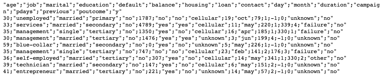
Figure 1.5: The first 10 rows of the dataset
Now let's load the data into memory using the pandas library with the read_csv function. First, import the pandas library:
import pandas as pd
bank_data = pd.read_csv('data/bank.csv', sep=';')
Finally, to verify that we have the data loaded into the memory correctly, we can print the first few rows. Then, print out the top 20 values of the variable:
bank_data.head(20)
The printed output should look like this:
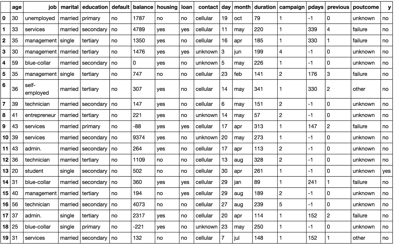
Figure 1.6: The first 20 rows of the pandas DataFrame
We can also print the shape of the DataFrame:
bank_data.shape
The printed output should look as follows, showing that the DataFrame has 4,521 rows and 17 columns:
The following figure shows the output of the preceding code:
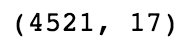
Figure 1.7: Output of the shape command on the DataFrame
We have successfully loaded the data into memory, and now we can manipulate and clean the data so that a model can be trained using this data. Remember that machine learning models require data to be represented as numerical data types in order to be trained. We can see from the first few rows of the dataset that some of the columns are string types, so we will have to convert them to numerical data types later in the chapter.
We can see that there is a given output variable for the dataset, known as 'y', which indicates whether or not the client has subscribed. This seems like an appropriate target to predict for, since it is conceivable that we may know all the variables about our clients, such as their age. For those variables that we don't know, substituting unknowns is acceptable. The 'y' target may be useful to the bank to figure out as to which customers they want to focus their resources on. We can create feature and target datasets as follows, providing the axis=1 argument:
feats = bank_data.drop('y', axis=1) target = bank_data['y']To verify that the shapes of the datasets are as expected, we can print out the number of rows and columns of each:
print(f'Features table has {feats.shape[0]} rows and {feats.shape[1]} columns')print(f'Target table has {target.shape[0]} rows')The following figure shows the output of the preceding code:
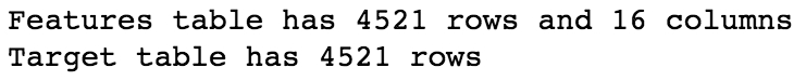
Figure 1.8: Output of the shape commands on the feature and target DataFrames
We can see two important things here that we should always verify before continuing: first, the number of rows of the feature DataFrame and target DataFrame are the same. Here, we can see that both have 4,521 rows. Second, the number of columns of the feature DataFrame should be one fewer than the total DataFrame, and the target DataFrame has exactly one column.
On the second point, we have to verify that the target is not contained in the feature dataset, otherwise the model will quickly find that this is the only column needed to minimize the total error, all the way down to zero. It's also not incredibly useful to include the target in the feature set. The target column doesn't necessarily have to be one column, but for binary classification, as in our case, it will be. Remember that these machine learning models are trying to minimize some cost function, in which the target variable will be part of that cost function.
Finally, we will save our DataFrames to CSV so that we can use them later:
feats.to_csv('data/bank_data_feats.csv')target.to_csv('data/bank_data_target.csv', header='y')