

While there are more than thirteen thousand packages in the CRAN repository, some of the packages have a unique place and utility for some major functionality. So far, we saw many examples of data manipulations such as join, aggregate, reshaping, and sub-setting. The R packages we will discuss next will provide a plethora of functions, providing a wide range of data processing and transformation capabilities.
The dplyr package helps in the most common data manipulation challenges through five different methods, namely, mutate(), select(), filter(), summarise(), and arrange(). Let's revisit our direct marketing campaigns (phone calls) of a Portuguese banking institution dataset from UCI Machine Learning Repository to test out all these methods.
The %>% symbol in the following exercise is called chain operator. The output of the one operation is sent to the next one without explicitly creating a new variable. Such a chaining operation is storage efficient and makes the readability of the code easy.
In this exercise, we are interested in knowing the average bank balance of people doing blue-collar jobs by their marital status. Use the functions from the dplyr package to get the answer.
Perform the following steps to complete the exercise:
Import the bank-full.csv file into the df_bank_detail object using the read.csv() function:
df_bank_detail <- read.csv("bank-full.csv", sep = ';')Now, load the dplyr library:
library(dplyr)
Select (filter) all the observations where the job column contains the value blue-collar and then group by the martial status to generate the summary statistic, mean:
df_bank_detail %>%
  filter(job == "blue-collar") %>%
  group_by(marital) %>%
  summarise(
    cnt = n(),
    average = mean(balance, na.rm = TRUE)
  )
The output is as follows:
## # A tibble: 3 x 3
##    marital   cnt   average
##     <fctr> <int>     <dbl>
## 1 divorced   750  820.8067
## 2  married  6968 1113.1659
## 3   single  2014 1056.1053
Let's find out the bank balance of customers with secondary education and default as yes:
df_bank_detail %>%
  mutate(sec_edu_and_default = ifelse((education == "secondary" & default == "yes"), "yes","no")) %>%
  select(age, job, marital,balance, sec_edu_and_default) %>%
  filter(sec_edu_and_default == "yes") %>%
  group_by(marital) %>%
  summarise(
    cnt = n(),
    average = mean(balance, na.rm = TRUE)
  )
The output is as follows:
## # A tibble: 3 x 3
##    marital   cnt    average
##     <fctr> <int>      <dbl>
## 1 divorced    64   -8.90625
## 2  married   243  -74.46914
## 3   single   151 -217.43046
Much of complex analysis is done with ease. Note that the mutate() method helps in creating custom columns with certain calculation or logic.
The tidyr package has three essential functions—gather(), separate(), and spread()—for cleaning messy data.
The gather() function converts wide DataFrame to long by taking multiple columns and gathering them into key-value pairs.
In this exercise, we will explore the tidyr package and the functions associated with it.
Perform the following steps to complete the exercise:
Import the tidyr library using the following command:
library(tidyr)
Next, set the seed to 100 using the following command:
set.seed(100)
Create an r_name object and store the 5 person names in it:
r_name <- c("John", "Jenny", "Michael", "Dona", "Alex")For the r_food_A object, generate 16 random numbers between 1 to 30 without repetition:
r_food_A <- sample(1:150,5, replace = FALSE)
Similarly, for the r_food_B object, generate 16 random numbers between 1 to 30 without repetition:
r_food_B <- sample(1:150,5, replace = FALSE)
Create and print the data from the DataFrame using the following command:
df_untidy <- data.frame(r_name, r_food_A, r_food_B)
df_untidy
The output is as follows:
##    r_name r_food_A r_food_B
## 1    John       47       73
## 2   Jenny       39      122
## 3 Michael       82       55
## 4    Dona        9       81
## 5    Alex       69       25
Use the gather() method from the tidyr package:
df_long <- df_untidy %>%
  gather(food, calories, r_food_A:r_food_B)
df_long
The output is as follows:
##     r_name     food calories
## 1     John r_food_A       47
## 2    Jenny r_food_A       39
## 3  Michael r_food_A       82
## 4     Dona r_food_A        9
## 5     Alex r_food_A       69
## 6     John r_food_B       73
## 7    Jenny r_food_B      122
## 8  Michael r_food_B       55
## 9     Dona r_food_B       81
## 10    Alex r_food_B       25
The spread() function works the other way around of gather(), that is, it takes a long format and converts it into wide format:
df_long %>%
  spread(food,calories)
##    r_name r_food_A r_food_B
## 1    Alex       69       25
## 2    Dona        9       81
## 3   Jenny       39      122
## 4    John       47       73
## 5 Michael       82       55
The separate() function is useful in places where columns are a combination of values and is used for making it a key column for other purposes. We can separate out the key if it has a common separator character:
key <- c("John.r_food_A", "Jenny.r_food_A", "Michael.r_food_A", "Dona.r_food_A", "Alex.r_food_A", "John.r_food_B", "Jenny.r_food_B", "Michael.r_food_B", "Dona.r_food_B", "Alex.r_food_B")
calories <- c(74, 139, 52, 141, 102, 134, 27, 94, 146, 20)
df_large_key <- data.frame(key,calories)
df_large_key
The output is as follows:
##                 key calories
## 1     John.r_food_A       74
## 2    Jenny.r_food_A      139
## 3  Michael.r_food_A       52
## 4     Dona.r_food_A      141
## 5     Alex.r_food_A      102
## 6     John.r_food_B      134
## 7    Jenny.r_food_B       27
## 8  Michael.r_food_B       94
## 9     Dona.r_food_B      146
## 10    Alex.r_food_B       20
df_large_key %>%
  separate(key, into = c("name","food"), sep = "\\.")
##       name     food calories
## 1     John r_food_A       74
## 2    Jenny r_food_A      139
## 3  Michael r_food_A       52
## 4     Dona r_food_A      141
## 5     Alex r_food_A      102
## 6     John r_food_B      134
## 7    Jenny r_food_B       27
## 8  Michael r_food_B       94
## 9     Dona r_food_B      146
## 10    Alex r_food_B       20
This activity will make you accustomed to selecting all numeric fields from the bank data and produce the summary statistics on numeric variables.
Perform the following steps to complete the activity:
Extract all numeric variables from bank data using select().
Using the summarise_all() method, compute min, 1st quartile, 3rd quartile, median, mean, max, and standard deviation.
Store the result in a DataFrame of wide format named df_wide.
Now, to convert wide format to deep, use the gather, separate, and spread functions of the tidyr package.
The final output should have one row for each variable and one column each of min, 1st quartile, 3rd quartile, median, mean, max, and standard deviation.
Once you complete the activity, you should have the final output as follows:
## # A tibble: 4 x 8
##        var   min   q25 median   q75    max       mean         sd
## *    <chr> <dbl> <dbl>  <dbl> <dbl>  <dbl>      <dbl>      <dbl>
## 1      age    18    33     39    48     95   40.93621   10.61876
## 2  balance -8019    72    448  1428 102127 1362.27206 3044.76583
## 3 duration     0   103    180   319   4918  258.16308  257.52781
## 4    pdays    -1    -1     -1    -1    871   40.19783  100.12875
What we saw with the apply functions could be done through the plyr package on a much bigger scale and robustness. The plyr package provides the ability to split the dataset into subsets, apply a common function to each subset, and combine the results into a single output. The advantage of using plyr over the apply function is features like the following:
Speed of code execution
Parallelization of processing using foreach loop
Support for list, DataFrame, and matrices
Better debugging of errors
All the function names in plyr are clearly defined based on input and output. For example, if an input is a DataFrame and output is list, the function name would be dlply.
The following figure from the The Split-Apply-Combine Strategy for Data Analysis paper displays all the different plyr functions:
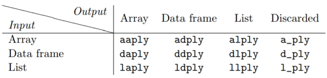
Figure 1.7: Functions in the plyr packages
The _ means the output will be discarded.
In this exercise, we will see how split-apply-combine makes things simple with the flexibility of controlling the input and output.
Perform the following steps to complete the exercise:
Load the plyr package using the following command:
library(plyr)
Next, use the slightly tweaked version of the c_vowel function we created in the earlier example in Exercise 13, Exploring the apply Function:
c_vowel <- function(x_char){
  return(sum(as.character(x_char[,"b"]) %in% c("A","I","O","U")))
}
Set the seed to 101:
set.seed(101)
Store the value in the r_characters object:
r_characters <- data.frame(a=rep(c("Split_1","Split_2","Split_3"),1000), b= sample(LETTERS, 3000, replace = TRUE))Use the dlply() function and print the split in the row format:
dlply(r_characters, c_vowel)
The output is as follows:
## $Split_1
## [1] 153
##
## $Split_2
## [1] 154
##
## $Split_3
## [1] 147
We can simply replace dlply with the daply() function and print the split in the column format as an array:
daply(r_characters, c_vowel)
The output is as follows:
## Split_1 Split_2 Split_3
##     153     154     147
Use the ddply() function and print the split:
ddply(r_characters, c_vowel)
The output is as follows:
##         a  V1
## 1 Split_1 153
## 2 Split_2 154
## 3 Split_3 147
In steps 5, 6, and 7, observe how we created a list, array, and data as an output for DataFrame input. All we must do is use a different function from plyr. This makes it easy to type cast between many possible combinations.
The caret package is particularly useful for building a predictive model, and it provides a structure for seamlessly following the entire process of building a predictive model. Starting from splitting data to training and testing dataset and variable importance estimation, we will extensively use the caret package in our chapters on regression and classification. In summary, caret provides tools for:
Data splitting
Pre-processing
Feature selection
Model training
Model tuning using resampling
Variable importance estimation
We will revisit the caret package with examples in Chapter 4, Regression, and Chapter 5, Classification.