
Before installing RStudio, you should install R on your computer. RStudio will then automatically search for your R installation.
RStudio is based on the R framework and it requires, at least, R version 2.11.1, but we highly recommend that you install the latest version. The latest version of R is 3.2.2, as of September 2015.
We assume that most readers are using Windows or Mac OS systems. The installation of R is pretty simple. Just go to http://cran.rstudio.com, download the proper version of R for your system, and install it using the default setting.
We would like to leave more space to talk about installing R on different Linux distributions. As there are a huge number of different Linux distributions out there, we will focus, in this book, on the most used one: Ubuntu.
CRAN hosts repositories for Debian and Ubuntu. To install the latest version of R, you should add the CRAN repository to your system.
The supported releases are: Utopic Unicorn (14.10), Trusty Tahr (14.04; LTS), Precise Pangolin (12.04; LTS), and Lucid Lynx (10.04; LTS). However, only the latest Long Term Support (LTS) is fully supported by the R framework development team.
We will take Ubuntu 14.04 LTS as an example. Perform the following steps:
Open a new terminal window.
Add the repository for Ubuntu 14.04 to the file
/etc/apt/sources.list:$ sudo sh –c "echo 'deb http://cran.rstudio.com/bin/linux/ubuntu trusty/'>>/etc/apt/sources.listThe Ubuntu archives on CRAN are signed with a key, which has the key ID,
E084DAB9. So, we have to add the key to our system:$ sudo apt-key adv –keyserver keyserver.ubuntu.com –recv-keys E084DAB9Update the system and repository:
$ sudo apt-get updateInstall R with:
$ sudo apt-get install r-baseInstall the developer package:
$ sudo apt-get install r-base-devInstalling RStudio
Installing RStudio on Windows and Ubuntu is pretty much the same, as RStudio offers installers for nearly all platforms. The steps are listed as follows:
Download the newest installer for your system.
Install RStudio using the default settings.
As R updates continuously, it is possible that you have, even after a short time, several versions of R installed on your system. Sometimes, you also have projects that require an older version of R to run properly.
When R is installed on Windows, it automatically writes the version being installed into the registry as the current version of R. And this will also be the version that RStudio uses. You can choose the version of R that you want to use by holding the Ctrl key during the launch of RStudio.
On Linux, you can use a command with R to see which version of R, RStudio uses. If you want RStudio to use another version of R (maybe you want to use an older version or because you had to install R in your Documents folder because of missing admin rights) you can overwrite the settings with the following export: RSTUDIO_WHICH_R=/usr/local/bin/R. This line has to be added to your ~/.profile file.
Updating RStudio is as easy as installing it. If you want to check if an update is available, navigate to Help | Check for Updates.
If an update is available, you can download the newest version and just install it. As RStudio saves all user information in the user's home directory, they will still be there after the update.

When you start RStudio for the first time, you will see four main panes. If you want to customize the four main panes, you can do it by navigating to Tools | Global Options | Pane Layout.
We will explain their use, but first we need to create a new R script file by clicking on File | New File | R Script.

The new R script file is opened in a new pane and is named Untitled1.

You can see that we now have four panes. They are named as follows:
RStudio's source editor was developed in a fully functional R editor over the last few years. It has a powerful syntax highlighter that works with not only every format connected to R development, such as R Scripts, R Markdown, or R documentation files, but also C++, JavaScript, HTML, and many more.
We've already created a new R script file and can now demonstrate some of the code editor's functions. You can also open an existing R document by clicking on File | Open File, or by using the shortcut, Ctrl + O.
The code editor works with tabs, which gives you the possibility of opening several files at the same time, as you can see in the following screenshot. If there are unsaved changes in a file, their names will be highlighted in red and marked with an asterisk.

If you have several files opened, you will see a double arrow in the menu of the source code editor. This will open a small menu showing you an overview of all the opened files. You can also search for a specific file.

Under the tabs with the opened files, you can see a toolbox with tools for the code editor. For example, you have the Source on Save checkbox. This is a really handy tool especially when you are working on a reusable function. If activated, the function is automatically sourced to the global environment and we do not have to source it manually again after editing the code.
Another function you can find in the toolbox is the search and replace tool. This is known from a lot of text editors and helps you find existing code and replace it. RStudio also offers different options for your search, such as In selection, to just search in the code you selected in the editor or Match case, to make the search case-sensitive. This is demonstrated in the following screenshot:

RStudio highlights parts of your code according to the R language definition. This makes your code much easier to read. The default settings are:
One of the most important menus in the source editor is what you find when you click on the magic stick. If you forgot what exact arguments the selected function needs, just hit the Tab button and you will see a list of available arguments with a description, if available:

You can then scroll through the list and select the argument you want to use. This is especially useful when you have functions that can be called with a lot of different arguments; it would be very time-consuming to open the package documentation for every function call.

You can also find direct links to the help or function definition, which shows you where the current function is defined.
After that, you can find the functions, Extract Function and Extract Variable. These functions help you in creating functions. When you click on Extract Function or use the shortcut, Ctrl + Alt + X, RStudio creates a function from your selection and inserts it in the source code.

After executing the command, your code will look like this:

The next button is the Compile Notebook button. This helps you compile your currently opened source file into a notebook with the format, HTML, PDF, or MS Word:

The compiled report will then open in a new window.

This is the code we used for the preceding example; if you want to reproduce it, type the following code:
x <- 10 + (1:20)/10
y <- x^2 + rnorm(length(x))
plot(x, y)
On the extreme right of the source code menu, you will find the buttons needed to run the code. These buttons are:
The Run button executes a single line and the shortcut is Ctrl + Enter
To re-run the previous region (Ctrl + Shift + P)
The Source button executes the entire source file (Ctrl + Shift + Enter)
Tip
Code regions are foldable regions of code in the code editor. We will explain later how you can create them.
If you want to execute a single line, or rather, if you want to run the current line where your cursor is, you can use the Run button or the shortcut, Ctrl + Enter. After the execution, the cursor will jump to the next line in the source file.
If you want to execute several lines of code, you can select the lines and press the Run button.
RStudio supports both automatic and user-defined folding for regions of code. This is a very handy feature, especially when you work with functions and larger scripts. It lets you hide and show blocks to make the code easier to navigate.
RStudio automatically folds the following regions in the source editor:
Braced regions (function definitions, conditional blocks, and so on)
Code chunks within R Sweave or R Markdown documents
Code sections (user-defined)
The output looks like this:

To define a code section on your own and to make it easier to navigate in larger source files, you can use three methods:
# Section One ----------------------
# Section Two =============
### Section Three #############
So, the line can start with any number of pound signs (#), but is has to end with at least four or more -, =, or # characters. RStudio then automatically defines the following code as the section. To navigate between code sections, you can use the Jump To menu at the bottom of the editor.

The menu at the bottom, on the right-hand side lets you choose the file format of the currently opened source file. Normally, RStudio chooses the right format automatically. If you change it manually, the code completion and the syntax highlighting will adapt to the new settings.

RStudio offers visual debuggers to help you understand code and find bugs and problems. Therefore, it uses the debugging functions of R but integrates them seamlessly into the RStudio user interface. You can find these tools in the Debug tab of the menu, or by pressing Alt + D:

You can set breakpoints right in the source editor by clicking on the number of the line, or by pressing Shift + F9:

The debugger output can help you find bugs in your code in a better way. In this example, the debugger output is debug.R:10. This means that we should look into the tenth line of the source file:

With the default settings, this pane consists of the tabs, Environment and History. You can use the shortcut, Ctrl + 8, to switch to the Environment browser, and Ctrl + 4 to switch to the History window:

The Environment pane is one of the biggest advantages of RStudio. It gives you an overview over all objects currently available in an environment. So, you can see a list of all data, values, and functions.
The Environment browser shows you the number of observations and the number of variables in the second column. If you want to get a better overview of a dataset, you can click on the table symbol at the end of the row.

When you click on the blue and white arrow next to the name of an object, you will see its structure. This is basically the output of the str() function, but in a more structured way.
The Import Dataset button offers you an easy way to import data. It basically uses the read.csv() function but offers you a graphical interface to set the parameters for the import. You can either import the dataset from a local file, or you can choose an import from a URL.

Furthermore, the Environment pane gives you the possibility of clearing the environment, which will delete all defined variables and also all sourced functions.
The History pane shows all the commands you entered in the console, and it also lets you send the selected command back from the history directly to the console with the To Console button or back to the opened source code file with the To Source button. You can also delete commands from the history by selecting them and pressing the paper icon with the red close sign above the history. Or you can clear the whole history by clicking the broom icon:

The console pane is basically an R console but it is enhanced with some RStudio functions. This includes the command completion known from the source editor, and a history popup, which shows you the recent commands you used.
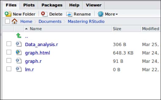
This pane is, like the name says, divided into five sub panes: Files, Plots, Packages, Help, and Viewer.
This pane is one of RStudio's biggest enhancements in comparison to the normal R console. The Files pane shows you all the files in the current working directory. It includes information about the file size and when the data was last modified. Clicking on an item will open it with the appropriate application.
The Plot pane in RStudio handles all of your graphics output. This makes working with graphical output much easier than in the regular R console, as it opens a new window for every graphic.

Furthermore, the Plot pane gives some more tools. These tools include the option to zoom into a graphic. This will open a new window with a bigger version of the current plot. This plot will then arrange itself to the current window size.
You can also export the current plotted graphic with the Export button. The Export menu has three options:

When you choose the Save as Image... option, RStudio will open a popup that lets you define the export image format, the directory, and the file name, as well as the width and height.

The Save as PDF... option will create a single page PDF document with your plot. Based on the width and height settings, it will be either in the landscape or portrait format.
RStudio also offers the option to publish your plots on RPubs. This is a free and very simple web service from the makers of RStudio to upload R graphics and R Markdown documents, which will then be publicly available on the web and you can share the link. We will talk about the possibilities of R markdown in a later chapter.
When you click on the Publish button, a window will open and guide you through the process.

After clicking on Publish, a new browser window will open and show your uploaded report:

The Package pane helps you install, update, or load packages. It gives you an overview about all installed packages, a short description, and the installed version.
If you tick a checkbox in front of a package, it will automatically be loaded, and if you remove the tick again, RStudio will automatically detach it from the environment. So, it basically unloads it again.
The Packages pane also provides a handy tool to install new packages with the help of a graphical interface. We just have to click on the Install button and we will be guided through the installation process. The Install packages dialog also allows us to install packages that we have saved locally on our computer:

You can see next what RStudio does in the R console:

A big advantage of the R language is that every package on CRAN will come with package documentation. You can find these files on the CRAN website but RStudio bundles them in a handy Help pane. You can search the help through the search bar, or you can just press F1:

The Viewer pane in RStudio can be used to view local web content, such as web graphics created with packages such as rCharts, googleVis, and others. It can also show local web applications created with Shiny or OpenCPU.

Now, we will click on Save as Web Page... in the Export menu.

The export menu of the viewer pane offers, basically, the same option to export your work but replaces the Save as image option with Save as Web Page. This creates a standalone web page.
The default options of RStudio are the best for most people, but you can also change the appearance and the pane layout completely according to your needs and wishes. We can open the Options menu by clicking on Tools | Global Options:

RStudio offers a lot of ways to personalize the code editing. We can, for example, set the spaces that will be inserted when we use the Tab key, or change the diagnostics information shown. You also have the Appearance tab, as shown next:

Here you can edit, for example, the font used in the code editor, or the editor theme. This way, you can make RStudio look the way you want it to.
And the Pane Layout tab: In this pane, we can change the content of the four main panes in the Pane Layout tab. You can make each of them a source, a console, or an individualized pane. So, the last option means that you can easily add elements to the pane with the help of the checkboxes.

The fastest way to use RStudio is by using it with keyboard shortcuts. In the previous text, we already mentioned some of them. But we put the most important ones together in a table, which is as follows:
|
Description |
Windows and Linux |
Mac |
|---|---|---|
|
Move the focus to the Source editor |
Ctrl + 1 |
Ctrl + 1 |
|
Move the focus to console |
Ctrl + 2 |
Ctrl + 2 |
|
Move the focus to Help |
Ctrl + 3 |
Ctrl + 3 |
|
Show the History pane |
Ctrl + 4 |
Ctrl +4 |
|
Show the Files pane |
Ctrl + 5 |
Ctrl +5 |
|
Show the Plots pane |
Ctrl + 6 |
Ctrl + 6 |
|
Show the Packages pane |
Ctrl + 7 |
Ctrl + 7 |
|
Show the Environment pane |
Ctrl + 8 |
Ctrl + 8 |
|
Open the document |
Ctrl + O |
Command + O |
|
Run the current line/section |
Ctrl + Enter |
Command + Enter |
|
Clear the console |
Ctrl + L |
Command + L |
|
Extract the function from the selection |
Ctrl + Alt + X |
Command + Option + X |
|
Ctrl + Shift + Enter |
Command + Shift + Enter | |
|
Toggle the breakpoint |
Shift + F9 |
Shift + F9 |