In this book, the models we will study have two important and defining characteristics. The first of these is that we will not use mathematical reasoning or logical induction to produce a model from known facts, nor will we build models from technical specifications or business rules; instead, the field of predictive analytics builds models from data. More specifically, we will assume that for any given predictive task that we want to accomplish, we will start with some data that is in some way related to or derived from the task at hand. For example, if we want to build a model to predict annual rainfall in various parts of a country, we might have collected (or have the means to collect) data on rainfall at different locations, while measuring potential quantities of interest, such as the height above sea level, latitude, and longitude. The power of building a model to perform our predictive task stems from the fact that we will use examples of rainfall measurements at a finite list of locations to predict the rainfall in places where we did not collect any data.

The second important characteristic of the problems for which we will build models is that during the process of building a model from some data to describe a particular phenomenon, we are bound to encounter some source of randomness. We will refer to this as the stochastic or nondeterministic component of the model. It may be the case that the system itself that we are trying to model doesn't have any inherent randomness in it, but it is the data that contains a random component. A good example of a source of randomness in data is the measurement of the errors from the readings taken for quantities such as temperature. A model that contains no inherent stochastic component is known as a deterministic model, Newton's Second Law being a good example of this. A stochastic model is one that assumes that there is an intrinsic source of randomness to the process being modeled. Sometimes, the source of this randomness arises from the fact that it is impossible to measure all the variables that are most likely impacting a system, and we simply choose to model this using probability. A well-known example of a purely stochastic model is rolling an unbiased six-sided die. Recall that in probability, we use the term random variable to describe the value of a particular outcome of an experiment or of a random process. In our die example, we can define the random variable, Y, as the number of dots on the side that lands face up after a single roll of the die, resulting in the following model:

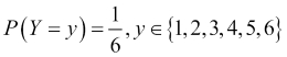
This model tells us that the probability of rolling a particular digit, say, three, is one in six. Notice that we are not making a definite prediction on the outcome of a particular roll of the die; instead, we are saying that each outcome is equally likely.

In the case of the die model, there aren't any variables that we have to measure. In most cases, however, we'll be looking at predictive models that involve a number of independent variables that are measured, and these will be used to predict a dependent variable. Predictive modeling draws on many diverse fields and as a result, depending on the particular literature you consult, you will often find different names for these. Let's load a data set into R before we expand on this point. R comes with a number of commonly cited data sets already loaded, and we'll pick what is probably the most famous of all, the iris data set:

> head(iris, n = 3)
  Sepal.Length Sepal.Width Petal.Length Petal.Width Species
1          5.1         3.5          1.4         0.2  setosa
2          4.9         3.0          1.4         0.2  setosa
3          4.7         3.2          1.3         0.2  setosa

The iris data set consists of measurements made on a total of 150 flower samples of three different species of iris. In the preceding code, we can see that there are four measurements made on each sample, namely the lengths and widths of the flower petals and sepals. The iris data set is often used as a typical benchmark for different models that can predict the species of an iris flower sample, given the four previously mentioned measurements. Collectively, the sepal length, sepal width, petal length, and petal width are referred to as features, attributes, predictors, dimensions, or independent variables in literature. In this book, we prefer to use the word feature, but other terms are equally valid. Similarly, the species column in the data frame is what we are trying to predict with our model, and so it is referred to as the dependent variable, output, or target. Again, in this book, we will prefer one form for consistency, and will use output. Each row in the data frame corresponding to a single data point is referred to as an observation, though it typically involves observing the values of a number of features.

As we will be using data sets, such as the iris data described earlier, to build our predictive models, it also helps to establish some symbol conventions. Here, the conventions are quite common in most of the literature. We'll use the capital letter, Y, to refer to the output variable, and subscripted capital letter, X_i, to denote the i^th feature. For example, in our iris data set, we have four features that we could refer to as X₁ through X₄. We will use lower case letters for individual observations, so that x₁ corresponds to the first observation. Note that x₁ itself is a vector of feature components, x_ij, so that x₁₂ refers to the value of the second feature in the first observation. We'll try to use double suffixes sparingly and we won't use arrows or any other form of vector notation for simplicity. Most often, we will be discussing either observations or features and so the case of the variable will make it clear to the reader which of these two is being referenced.

When thinking about a predictive model using a data set, we are generally making the assumption that for a model with n features, there is a true or ideal function, f, that maps the features to the output:

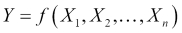
We'll refer to this function as our target function. In practice, as we train our model using the data available to us, we will produce our own function that we hope is a good estimate for the target function. We can represent this by using a caret on top of the symbol f to denote our predicted function, and also for the output, Y, since the output of our predicted function is the predicted output. Our predicted output will, unfortunately, not always agree with the actual output for all observations (in our data or in general):

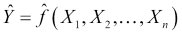
Given this, we can essentially summarize the process of predictive modeling as a process that produces a function to predict a quantity, while minimizing the error it makes compared to the target function. A good question we can ask at this point is, where does the error come from? Put differently, why are we generally not able to exactly reproduce the underlying target function by analyzing a data set?

The answer to this question is that in reality there are several potential sources of error that we must deal with. Remember that each observation in our data set contains values for n features, and so we can think about our observations geometrically as points in an n-dimensional feature space. In this space, our underlying target function should pass through these points by the very definition of the target function. If we now think about this general problem of fitting a function to a finite set of points, we will quickly realize that there are actually infinite functions that could pass through the same set of points. The process of predictive modeling involves making a choice in the type of model that we will use for the data thereby constraining the range of possible target functions to which we can fit our data. At the same time, the data's inherent randomness cannot be removed no matter what model we select. These ideas lead us to an important distinction in the types of error that we encounter during modeling, namely the reducible error and the irreducible error respectively.

The reducible error essentially refers to the error that we as predictive modelers can minimize by selecting a model structure that makes valid assumptions about the process being modeled and whose predicted function takes the same form as the underlying target function. For example, as we shall see in the next chapter, a linear model imposes a linear relationship between the features in order to compose the output. This restrictive assumption means that no matter what training method we use, how much data we have, and how much computational power we throw in, if the features aren't linearly related in the real world, then our model will necessarily produce an error for at least some possible observations. By contrast, an example of an irreducible error arises when trying to build a model with an insufficient feature set. This is typically the norm and not the exception. Often, discovering what features to use is one of the most time consuming activities of building an accurate model.

Sometimes, we may not be able to directly measure a feature that we know is important. At other times, collecting the data for too many features may simply be impractical or too costly. Furthermore, the solution to this problem is not simply an issue of adding as many features as possible. Adding more features to a model makes it more complex and we run the risk of adding a feature that is unrelated to the output thus introducing noise in our model. This also means that our model function will have more inputs and will, therefore, be a function in a higher dimensional space. Some of the potential practical consequences of adding more features to a model include increasing the time it will take to train the model, making convergence on a final solution harder, and actually reducing model accuracy under certain circumstances, such as with highly correlated features. Finally, another source of an irreducible error that we must live with is the error in measuring our features so that the data itself may be noisy.

Reducible errors can be minimized not only through selecting the right model but also by ensuring that the model is trained correctly. Thus, reducible errors can also come from not finding the right specific function to use, given the model assumptions. For example, even when we have correctly chosen to train a linear model, there are infinitely many linear combinations of the features that we could use. Choosing the model parameters correctly, which in this case would be the coefficients of the linear model, is also an aspect of minimizing the reducible error. Of course, a large part of training a model correctly involves using a good optimization procedure to fit the model. In this book, we will at least give a high level intuition of how each model that we study is trained. We generally avoid delving deep into the mathematics of how optimization procedures work but we do give pointers to the relevant literature for the interested reader to find out more.

So far we've established some central notions behind models and a common language to talk about data. In this section, we'll look at what the core components of a statistical model are. The primary components are typically:

As we'll see in this book, most models, such as neural networks, linear regression, and support vector machines have certain parameterized equations that describe them. Let's look at a linear model attempting to predict the output, Y, from three input features, which we will call X¹, X², and X³:

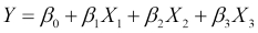
This model has exactly one equation describing it and this equation provides the linear structure of the model. The equation is parameterized by four parameters, known as coefficients in this case, and they are the four β parameters. In the next chapter, we will see exactly what roles these play, but for this discussion, it is important to note that a linear model is an example of a parameterized model. The set of parameters is typically much smaller than the amount of data available.

Given a set of equations and some data, we then talk about training the model. This involves assigning values to the model's parameters so that the model describes the data more accurately. We typically employ certain standard measures that describe a model's goodness of fit to the data, which is how well the model describes the training data. The training process is usually an iterative procedure that involves performing computations on the data so that new values for the parameters can be computed in order to increase the model's goodness of fit. For example, a model can have an objective or error function. By differentiating this and setting it to zero, we can find the combination of parameters that give us the minimum error. Once we finish this process, we refer to the model as a trained model and say that the model has learned from the data. These terms are derived from the machine learning literature, although there is often a parallel made with statistics, a field that has its own nomenclature for this process. We will mostly use the terms from machine learning in this book.

In order to put some of the ideas in this chapter into perspective, we will present our first model for this book, k-nearest neighbors, which is commonly abbreviated as kNN. In a nutshell, this simple approach actually avoids building an explicit model to describe how the features in our data combine to produce a target function. Instead, it relies on the notion that if we are trying to make a prediction on a data point that we have never seen before, we will look inside our original training data and find the k observations that are most similar to our new data point. We can then use some kind of averaging technique on the known value of the target function for these k neighbors to compute a prediction. Let's use our iris data set to understand this by way of an example. Suppose that we collect a new unidentified sample of an iris flower with the following measurements:

> new_sample
Sepal.Length  Sepal.Width Petal.Length  Petal.Width 
4.8          2.9          3.7          1.7

We would like to use the kNN algorithm in order to predict which species of flower we should use to identify our new sample. The first step in using the kNN algorithm is to determine the k-nearest neighbors of our new sample. In order to do this, we will have to give a more precise definition of what it means for two observations to be similar to each other. A common approach is to compute a numerical distance between two observations in the feature space. The intuition is that two observations that are similar will be close to each other in the feature space and therefore, the distance between them will be small. To compute the distance between two observations in the feature space, we often use the Euclidean distance, which is the length of a straight line between two points. The Euclidean distance between two observations, x¹ and x², is computed as follows:

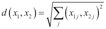
Recall that the second suffix, j, in the preceding formula corresponds to the j^th feature. So, what this formula is essentially telling us is that for every feature, take the square of the difference in values of the two observations, sum up all these squared differences, and then take the square root of the result. There are many other possible definitions of distance, but this is one of the most frequently encountered in the kNN setting. We'll see more distance metrics in Chapter 11, Recommendation Systems.

In order to find the nearest neighbors of our new sample iris flower, we'll have to compute the distance to every point in the iris data set and then sort the results. First, we'll begin by subsetting the iris data frame to include only our features, thus excluding the species column, which is what we are trying to predict. We'll then define our own function to compute the Euclidean distance. Next, we'll use this to compute the distance to every iris observation in our data frame using the apply() function. Finally, we'll use the sort() function of R with the index.return parameter set to TRUE, so that we also get back the indexes of the row numbers in our iris data frame corresponding to each distance computed:

> iris_features <- iris[1:4]
> dist_eucl <- function(x1, x2) sqrt(sum((x1 - x2) ^ 2))
> distances <- apply(iris_features, 1,
                     function(x) dist_eucl(x, new_sample))
> distances_sorted <- sort(distances, index.return = T)


> str(distances_sorted)
List of 2
 $ x : num [1:150] 0.574 0.9 0.9 0.949 0.954 ...
 $ ix: int [1:150] 60 65 107 90 58 89 85 94 95 99 ...

The $x attribute contains the actual values of the distances computed between our sample iris flower and the observations in the iris data frame. The $ix attribute contains the row numbers of the corresponding observations. If we want to find the five nearest neighbors, we can subset our original iris data frame using the first five entries from the $ix attribute as the row numbers:

> nn_5 <- iris[distances_sorted$ix[1:5],]
> nn_5
    Sepal.Length Sepal.Width Petal.Length Petal.Width    Species
60           5.2         2.7          3.9         1.4 versicolor
65           5.6         2.9          3.6         1.3 versicolor
107          4.9         2.5          4.5         1.7 virginica
90           5.5         2.5          4.0         1.3 versicolor
58           4.9         2.4          3.3         1.0 versicolor

As we can see, four of the five nearest neighbors to our sample are the versicolor species, while the remaining one is the virginica species. For this type of problem where we are picking a class label, we can use a majority vote as our averaging technique to make our final prediction. Consequently, we would label our new sample as belonging to the versicolor species. Notice that setting the value of k to an odd number is a good idea, because it makes it less likely that we will have to contend with tie votes (and completely eliminates ties when the number of output labels is two). In the case of a tie, the convention is usually to just resolve it by randomly picking among the tied labels. Notice that nowhere in this process have we made any attempt to describe how our four features are related to our output. As a result, we often refer to the kNN model as a lazy learner because essentially, all it has done is memorize the training data and use it directly during a prediction. We'll have more to say about our kNN model, but first we'll return to our general discussion on models and discuss different ways to classify them.