
R is a statistical programming language designed and created by Ross Ihaka and Robert Gentleman. It is a derivative of the S language created at the AT&T Bell laboratories. Apart from statistical analysis, R also supports powerful visualizations. It is open source, freely distributed under a General Public License (GPL). Comprehensive R Archive Network (CRAN) is an ever-growing repository with more than 8,400 packages, which can be freely installed and used for various kinds of analysis.
R is a high-level language based on interpretations and intuitive syntax. It runs on system's or server's active memory (RAM) and stores all files, functions, and derived results in its environment as objects. The architecture utilized in R computation is shown in Figure 1.5:
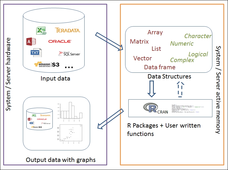
Figure 1.5: Illustrate architecture of R in local/server mode
R can be installed on any operating system, such as Windows, Mac OS X, and Linux. The installation files of the most recent version can be downloaded from any one of the mirror sites of CRAN: https://cran.r-project.org/. It is available under both 32-bit and 64-bit architectures.
The installation of r-base-dev is also highly recommended as it has many built-in functions. It also enables us to install and compile new R packages directly from the R console using the install.packages() command.
Upon installation, R can be called from program files, desktop shortcut, or from the command line. With default settings, the R console looks as follows:
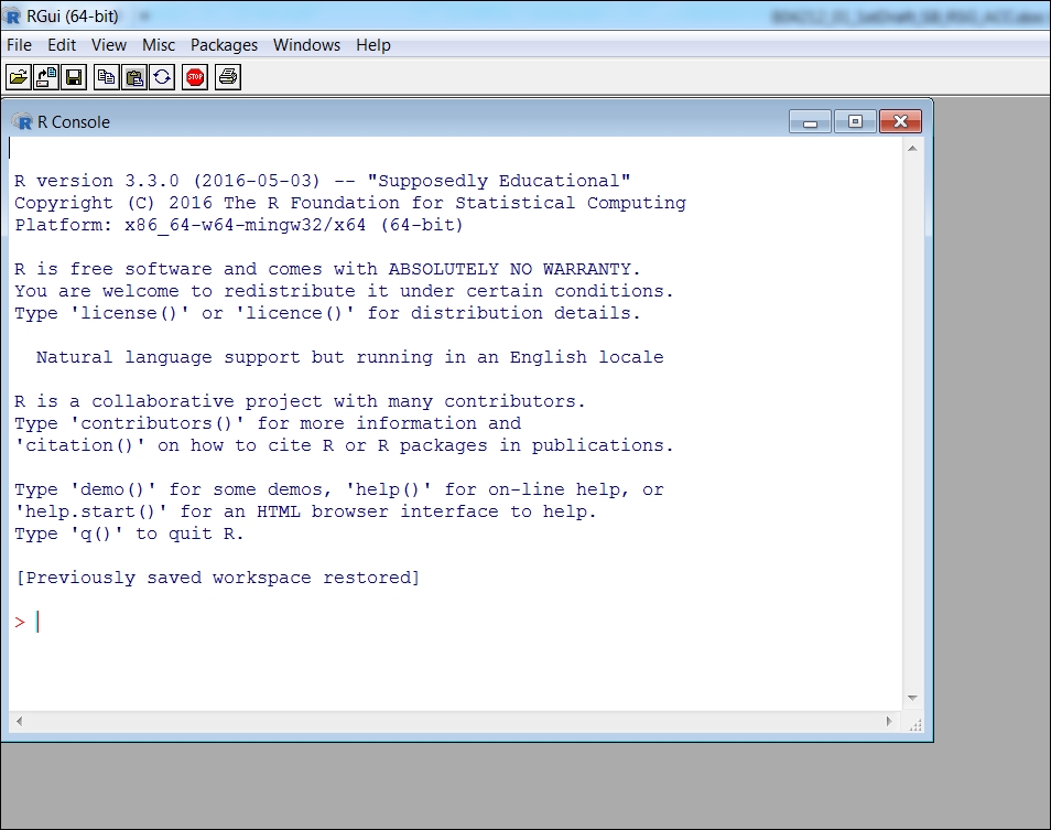
Figure 1.6: The R console in which one can start coding and evaluate results instantly
R can also be used as a kernel within Jupyter Notebook. Jupyter Notebook is a web-based application that allows you to combine documentation, output, and code. Jupyter can be installed using pip:
pip3 install -upgrade pip
pip3 install jupyter
To start Jupyter Notebook, open a shell/terminal and run this command to start the Jupyter Notebook interface in your browser:
jupyter notebook
To start a new R Notebook, click on right hand side New tab and select R kernel as shown in Figure 1.7. R kernel does not come as default in Jupyter Notebook with Python as prerequisite. Anaconda distribution is recommended to install python and Jupyter and can be downloaded from https://www.continuum.io/downloads. R essentials can be installed using below command.
conda install -c r r-essentials
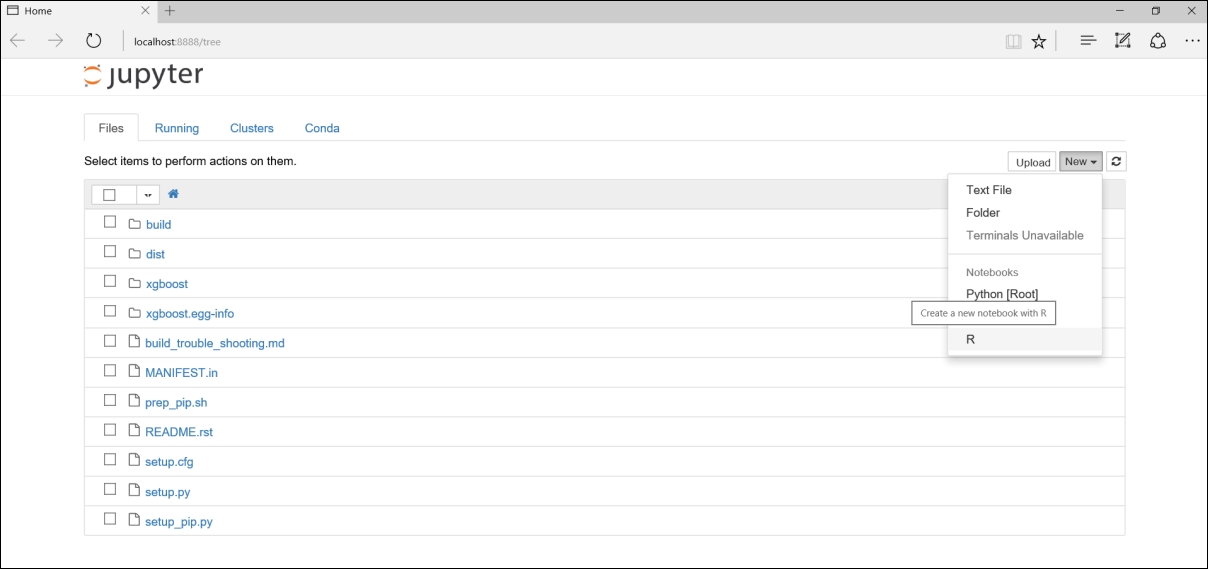
Figure 1.7: Jupyter Notebook for creating R notebooks
Once notebook is opened, you could start organizing your code into cells. As R does not require formal compilation, and executes codes on runtime, one can start coding and evaluate instant results. The console view can be modified using some options under the Windows tab. However, it is highly recommended to use an Integrated Development Environment (IDE), which would provide a powerful and productive user interface for R. One such widely used IDE is RStudio, which is free and open source. It comes with its own server (RStudio Server Pro) too. The interface of RStudio is as seen in the following screenshot:
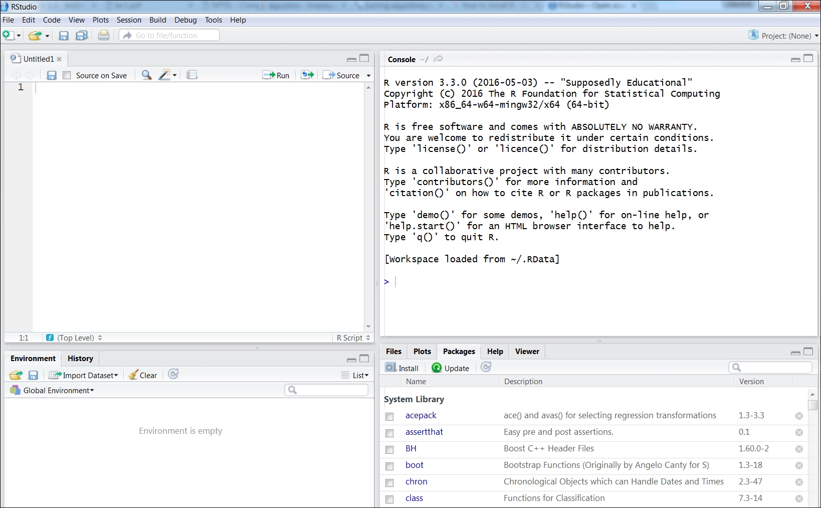
Figure 1.8: RStudio, a widely used IDE for R
R supports multiple types of data, which can be organized by dimensions and content type (homogeneous or heterogeneous), as shown in Table 1.1:
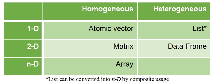
Table 1.1 Basic data structure in R
Homogeneous data structure is one which consists of the same content type, whereas heterogeneous data structure supports multiple content types. All other data structures, such as data tables, can be derived using these foundational data structures. Data types and their properties will be covered in detail in Chapter 3, Linked Lists.
The syntax of operators in R is very similar to other programming languages. The following is a list of operators along with their explanations.
The following table defines the various arithmetic operators:
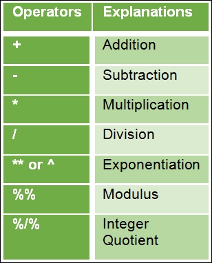
Table 1.2 Basic arithmetic operators in R
The following table defines the various logical operators:
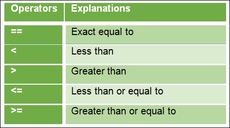
Table 1.3 Basic logical operators in R
An example of assigned in R is shown below. Initially a column vector V is assigned followed by operations on column vector such as addition, subtraction, square root and log. Any operation applied on column vector is element-wise operation.
> V <- c(1,2,3,4,5,6)  ## Assigning a vector V
> V
[1] 1 2 3 4 5 6
> V+10 ## Adding each element in vector V with 10
[1] 11 12 13 14 15 16
> V-1  ## Subtracting each element in vector V with 1
[1] 0 1 2 3 4 5
> sqrt(V)  ## Performing square root operation on each element in  vector V
[1] 1.000000 1.414214 1.732051 2.000000 2.236068 2.449490
> V1 <- log(V)  ## Storing log transformed of vector V as V1
> V1
[1] 0.0000000 0.6931472 1.0986123 1.3862944 1.6094379 1.7917595
Control structures such as loops and conditions form an integral part of any programming language, and R supports them with much intuitive syntax.
The syntax for the if condition is as follows:
    if (test expression)
    {
      Statement upon condition is true
    }
If the test expression is true, the statement is executed. If the statement is false, nothing happens.
In the following example, an atomic vector x is defined, and it is subjected to two conditions separately, that is, whether x is greater than 5 or less than 5. If either of the conditions gets satisfied, the value x gets printed in the console following the corresponding if statement:
> x <- 10
> if (x < 5) print(x)
> if (x > 5) print(x)
[1] 10
The syntax for the if...else condition is as follows:
    if(test expression)
    {
      Statement upon condition is true
    } else {
      Statement upon condition is false
    }
In this scenario, if the condition in the test expression is true, the statement under the if condition is executed, otherwise the statement under the else condition is executed.
The following is an example in which we define an atomic vector x with a value 10. Then, we verify whether x, when divided by 2, returns 1 (R reads 1 as a Boolean True). If it is True, the value x gets printed as an odd number, else as an even number:
> x=10
> if (x %% 2)
+ {
+   print(paste0(x, " :odd number"))
+ } else {
+   print(paste0(x, " :even number"))
+ }
[1] "10 :even number"
An ifelse() function is a condition used primarily for vectors, and it is an equivalent form of the if...else statement. Here, the conditional function is applied to each element in the vector individually. Hence, the input to this function is a vector, and the output obtained is also a vector. The following is the syntax of the ifelse condition:
    ifelse (test expression, statement upon condition is true,
    statement upon condition is false)
In this function, the primary input is a test expression which must provide a logical output. If the condition is true, the subsequent statement is executed, else the last statement is executed.
The following is example in which a vector x is defined with integer values from 1 to 7. Then, a condition is applied on each element in vector x to determine whether the element is an odd number or an even number:
> x <- 1:6
> ifelse(x %% 2, paste0(x, " :odd number"), paste0(x, " :even  number"))
[1] "1 :odd number"  "2 :even number" "3 :odd number"
[4] "4 :even number" "5 :odd number"  "6 :even number"
A for loop is primarily used to iterate a statement over a vector of values in a given sequence. The vector can be of any type, that is, numeric, character, Boolean, or complex. For every iteration, the statement is executed.
The following is the syntax of the for loop:
    for(x in sequence vector)
    {
      Statement to be iterated
    }
The loop continues till all the elements in the vector get exhausted as per the given sequence.
The following example details a for loop. Here, we assign a vector x, and each element in vector x is printed in the console using a for loop:
> x <- c("John", "Mary", "Paul", "Victoria")
> for (i in seq(x)) {
+   print(x[i])
+ }
[1] "John"
[1] "Mary"
[1] "Paul"
[1] "Victoria"
The nested for loop can be defined as a set of multiple for loops within each for loop as shown here:
    for( x in sequence vector)
    {
      First statement to be iterated
      for(y in sequence vector)
    {
      Second statement to be iterated
      .........
    }
  }
In a nested for loop, each subsequent for loop is iterated for all the possible times based on the sequence vector in the previous for loop. This can be explained using the following example, in which we define mat as a matrix (3x3), and our desired objective is to obtain a series of summations which will end up with the total sum of all the values within the matrix. Firstly, we initialize sum to 0, and then subsequently, sum gets updated by adding itself to all the elements in the matrix in a sequence. The sequence is defined by the nested for loop, wherein for each row in a matrix, each of the values in all the columns gets added to sum:
> mat <- matrix(1:9, ncol = 3)
> sum <- 0
> for (i in seq(nrow(mat)))
+ {
+   for (j in seq(ncol(mat)))
+   {
+     sum <- sum + mat[i, j]
+     print(sum)
+   }
+ }
[1] 1
[1] 5
[1] 12
[1] 14
[1] 19
[1] 27
[1] 30
[1] 36
[1] 45
In R, while loops are iterative loops with a specific condition which needs to be satisfied. The syntax of the while loop is as follows:
    while (test expression)
   {
     Statement upon condition is true (iteratively)
   }
Let's understand the while loop in detail with an example. Here, an object i is initialized to 1. The test expression which needs to be satisfied for every iteration is i<10. Since i = 1, the condition is TRUE, and the statement within the while loop is evaluated. According to the statement, i is printed on the console, and then increased by 1 unit. Now i increments to 2, and once again, the test expression, whether the condition (i < 10) is true or false, is checked. If TRUE, the statement is again evaluated. The loop continues till the condition becomes false, which, in our case, will happen when i increments to 10. Here, incrementing i becomes very critical, without which the loop can turn into infinite iterations:
> i <- 1
> while (i < 10)
+ {
+   print(i)
+   i <- i + 1
+ }
[1] 1
[1] 2
[1] 3
[1] 4
[1] 5
[1] 6
[1] 7
[1] 8
[1] 9
In R, the loops can be altered using break or next statements. This helps in inducing other conditions required within the statement inside the loop.
The syntax for the Break statement is break. It is used to terminate a loop and stop the remaining iterations. If a break statement is provided within a nested loop, then the innermost loop within which the break statement is mentioned gets terminated, and iterations of the outer loops are not affected.
The following is an example in which a for loop is terminated when i reaches the value 8:
> for (i in 1:30)
+ {
+   if (i < 8)
+   {
+     print(paste0("Current value is ",i))
+   } else {
+     print(paste0("Current value is ",i," and the loop breaks"))
+     break
+   }
+ }
[1] "Current value is 1"
[1] "Current value is 2"
[1] "Current value is 3"
[1] "Current value is 4"
[1] "Current value is 5"
[1] "Current value is 6"
[1] "Current value is 7"
[1] "Current value is 8 and the loop breaks"
The syntax for a Next statement is next. The next statements are used to skip intermediate iterations within a loop based on a condition. Once the condition for the next statement is met, all the subsequent operations within the loop get terminated, and the next iteration begins.
This can be further explained using an example in which we print only odd numbers based on a condition that the printed number, when divided by 2, leaves the remainder 1.
> for (i in 1:10)
+ {
+   if (i %% 2)
+   {
+     print(paste0(i, " is an odd number."))
+   } else {
+     next
+   }
+ }
[1] "1 is an odd number."
[1] "3 is an odd number."
[1] "5 is an odd number."
[1] "7 is an odd number."
[1] "9 is an odd number."
The repeat loop is an infinite loop which iterates multiple times without any inherent condition. Hence, it becomes mandatory for the user to explicitly mention the terminating condition, and use a break statement to terminate the loop.
The following is the syntax for a repeat statement:
    repeat
    {
      Statement to iterate along with explicit terminate condition
      including break statement
    }
In the current example, i is initialized to 1. Then, a for loop iterates, within which an object cube is evaluated and verified using a condition whether the cube is greater than 729 or not. Simultaneously, i is incremented by 1 unit. Once the condition is met, the for loop is terminated using a break statement:
> i <- 1
> repeat
+ {
+   cube <- i ** 3
+   i <- i + 1
+   if (cube < 729)
+   {
+     print(paste0(cube, " is less than 729. Let's remain in the
      loop."))
+   } else {
+     print(paste0(cube, " is greater than or equal to 729. Let's exit
      the loop."))
+     break
+   }
+ }
[1] "1 is less than 729. Let's remain in the loop."
[1] "8 is less than 729. Let's remain in the loop."
[1] "27 is less than 729. Let's remain in the loop."
[1] "64 is less than 729. Let's remain in the loop."
[1] "125 is less than 729. Let's remain in the loop."
[1] "216 is less than 729. Let's remain in the loop."
[1] "343 is less than 729. Let's remain in the loop."
[1] "512 is less than 729. Let's remain in the loop."
[1] "729 is greater than 729. Let's exit the loop."