
Now that we have our software installed and configured, we can focus on collecting some open source data. Data collecting (or data capture) is one of the key expertise of a GIS professional and it often covers a major part of a project budget. Surveying is expensive (for example, equipment, amortization, staff, and so on); however, buying data can also be quite costly. On the other hand, there is open and free data out there, which can drastically reduce the cost of basic analysis. It has some drawbacks, though. For example, the licenses are much harder to attune with commercial activity, because some of them are more restrictive.
There are two types of data collection. The first one is primary data collection, where we measure spatial phenomena directly. We can measure the locations of different objects with GPS, the elevation with radar or lidar, the land cover with remote sensing. There are truly a lot of ways of data acquisition with different equipment. The second type is secondary data collection, where we convert already existing data for our use case. A typical secondary data collection method is digitizing objects from paper maps. In this section, we will acquire some open source primary data.
Note
If you do not feel like downloading anything from the following data sources, you can work with the sample dataset of this book. The sample covers Luxembourg, therefore you can download and visualize it in no time.
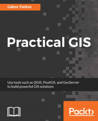
The only thing to consider is our study area. We should choose a relatively small administrative division, like a single county. For example, I'm choosing the county I live in as I'm quite familiar with it and it's small enough to make further analysis and visualization tasks fast and simple:
Note
Make sure you create a folder for the files that we will download. You should extract every dataset in a different folder with a talkative name to keep a clean working directory and to ease future work.
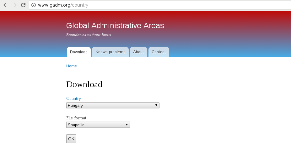
The first data we will download is the administrative boundaries of our country of choice. Open data for administrative divisions are easy to find for the first two levels, but it becomes more and more scarce for higher levels. The first level is always the countries' boundaries, while higher levels depend on the given country. There is a great source for acquiring the first three levels for every country in a fine resolution: GADM or Global Administrative Areas. We will talk about administration levels in more details in a later chapter. Let's download some data from http://www.gadm.org/country by selecting our study area, and the file format as Shapefile:
In the zipped archive, we will need the administrative boundaries, which contain our division of choice. If you aren't sure about the correct dataset, just extract everything and we will choose the correct one later.
The second vector dataset we download is the GeoNames archive for the country encasing our study area. GeoNames is a great place for finding data points. Every record in the database is a single point with a pair of coordinates and a lot of attribute data. Its most instinctive use case is for geocoding (linking names to locations). However, it can be a real treasure box for those who can link the rich attribute data to more meaningful objects. The country-level data dumps can be reached at http://download.geonames.org/export/dump/ through the countries' two-letter ISO codes.
Note
ISO (International Organization of Standards) is a large-scale organization maintaining a lot of standards for a wide variety of use cases. Country names also have ISO abbreviations, which can be reached at http://www.geonames.org/countries/ in the form of a list. The first column contains the two-letter ISO codes of the countries.
GADM's license is very restrictive. We are free to use the downloaded data for personal and research purposes but we cannot redistribute it or use it in commercial settings. Technically, it isn't open source data as it does not give the four freedoms of using, modifying, redistributing the original version, and redistributing the modified version without restrictions. That's why the example dataset doesn't contain GADM's version of Luxembourg.
Note
There is another data source, called Natural Earth, which is truly open source but it offers data only for the first two levels and on a lower resolution. If you need some boundaries with the least effort, make sure you check it out at http://www.naturalearthdata.com/downloads/.
GeoNames has two datasets--a commercially licensed premium dataset and an open source one. The open source data can be used for commercial purposes without restrictions.
Data acquisition with instruments mounted on airborne vehicles is commonly called remote sensing. Mounting sensors on satellites is a common practice by space agencies (for example, NASA and ESA), and other resourceful companies. These are also the main source of open source data as both NASA and ESA grant free access to preprocessed data coming from these sensors. In this part of the book, we will download remote sensing data (often called imagery) from USGS's portal: Earth Explorer. It can be found at https://earthexplorer.usgs.gov/. As the first step, we have to register an account in order to download data.
Note
If you would like to download Sentinel-2 data instead of Landsat imagery, you can find ESA's Copernicus data portal at https://scihub.copernicus.eu/.
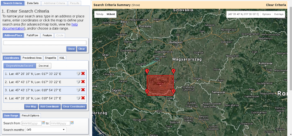
When we have an account, we should proceed to the Earth Explorer application and select our study area. We can select an area on the map by holding down the Shift button and drawing a rectangle with the mouse, as shown in the following screenshot:
As the next step, we should select some data from the Data Sets tab. There are two distinct types of remote sensing based on the type of sensor: active and passive. In active remote sensing, we emit some kind of signal from the instrument and measure its reflectance from the target surface. We make our measurement from the attributes of the reflected signal. Three very typical active remote sensing instruments are radar (radio detection and ranging) using radio waves, lidar (light detection and ranging) using laser, and sonar (sound navigation and ranging) using sound waves. The first dataset we download is SRTM (Shuttle Radar Topographic Mission), which is a DEM (digital elevation model) produced with a radar mounted on a space shuttle.
For this, we select the Digital Elevation item and then SRTM. Under the SRTM menu, there are some different datasets from which we need the 1 Arc-Second Global. Finally, we push the Results button, which navigates us to the results of our query. In the results window, there are quite a few options for every item, as shown in the following screenshot:
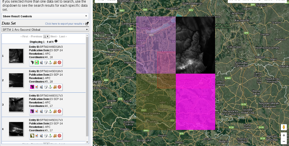
The first two options (Show Footprint and Show Browse Overlay) are very handy tools to show the selected imagery on the map. The footprint only shows the enveloping rectangle of the data, therefore, it is fast. Additionally, it colors every footprint differently, so we can identify them easily. The overlay tool is handy for getting a glance at the data without downloading it.
Finally, we download the tiles covering our study area. We can download them individually with the item's fifth option called Download Options. This offers some options from which we should select the BIL format as it has the best compression rate, thus, our download will be fast.
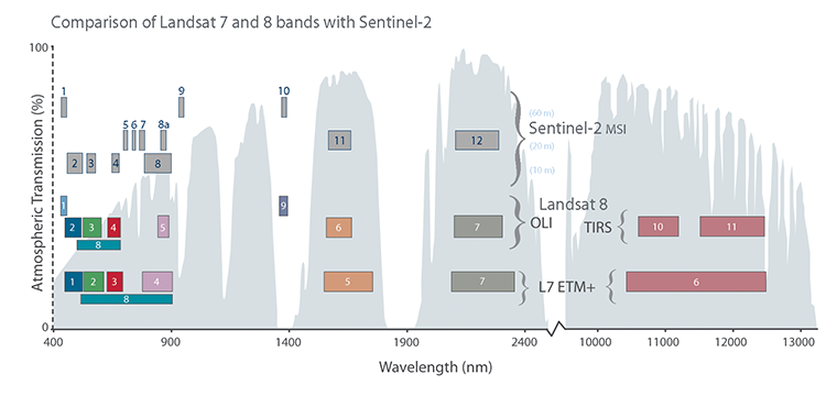
Let's get back to the Data Sets tab and select the next type of data we need to download--the Landsat data. These are measured with instruments of the other type--passive remote sensing. In passive remote sensing, we don't emit any signal, just record the electromagnetic radiance of our environment. This method is similar to the one used by our digital cameras except those record only the visible spectrum (about 380-450 nanometers) and compose an RGB picture from the three visible bands instantly. The Landsat satellites use radiometers to acquire multispectral images (bands). That is, they record images from spectral intervals, which can penetrate the atmosphere, and store each of them in different files. There is a great chart created by NASA (http://landsat.gsfc.nasa.gov/sentinel-2a-launches-our-compliments-our-complements/) which illustrates the bands of Landsat 7, Landsat 8, and Sentinel-2 along with the atmospheric opacity of the electromagnetic spectrum:
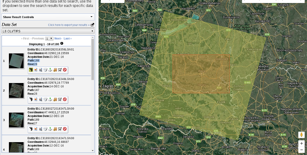
From the Landsat Archive, we need the Pre-Collection menu. From there, we select L8 OLI/TIRS and proceed to the results. With the footprints of the items, let's select an image which covers our study area. As Landsat images have a significant amount of overlap, there should be one image which, at least, mostly encases our study area. There are two additional information listed in every item--the row number and the path number. As these kinds of satellites are constantly orbiting Earth, we should be able to use their data for detecting changes. To assess this kind of use case (their main use case), their orbits are calculated so that, the satellites return to the same spot periodically (in case of Landsat, 18 days). This is why we can classify every image by their path and row information:
Note
To make sure the images are illuminated the same way every time on a given path/row, this kind of satellite is set on a Sun-synchronous orbit. This means, they see the same spot at the same solar time in every pass. There is a great video created by NASA visualizing Landsat's orbit at https://www.youtube.com/watch?v=P-lbujsVa2M.
Let's note down the path and row information of the selected imagery and go to the Additional Criteria tab. We feed the path and row information to the WRS Path and WRS Row fields and go back to the results. Now the results are filtered down, which is quite convenient as the images are strongly affected by weather and seasonal effects. Let's choose a nice imagery with minimal cloud coverage and download its Level 1 GeoTIFF Data Product. From the archive, we will need the TIFF files of bands 1-6.
SRTM is in the public domain; therefore, it can be used without restrictions, and giving attribution is also optional. Landsat data is also open source; however, based on USGS's statement (https://landsat.usgs.gov/are-there-any-restrictions-use-or-redistribution-landsat-data), proper attribution is recommended.
The last dataset we put our hands on is the swiss army knife of open source GIS data. OpenStreetMap provides vector data with a great global coverage coming from measurements of individual contributors. OpenStreetMap has a topological structure; therefore, it's great for creating beautiful visualizations and routing services. On the other hand, its collaborative nature makes accuracy assessments hard. There are some studies regarding the accuracy of the whole data, or some of its subsets, but we cannot generalize those results as accuracy can greatly vary even in small areas.
One of the main strengths of OpenStreetMap data is its large collection and variety of data themes. There are administrative borders, natural reserves, military areas, buildings, roads, bus stops, even benches in the database. Although its data isn't surveyed with geodesic precision, its accuracy is good for a lot of cases: from everyday use to small-scale analysis where accuracy in the order of meters is good enough (usually, a handheld GPS has an accuracy of under 5 meters). Its collaborative nature can also be evaluated as a strength as mistakes are corrected rapidly and the content follows real-world changes (especially large ones) with a quick pace.
Accessing OpenStreetMap data can be tricky. There are some APIs and other means to query OSM, although either we need to know how to code or we get everything in one big file. There is one peculiar company which creates thematic data extracts from the actual content--Geofabrik. We can reach Geofabrik's download portal at http://download.geofabrik.de/. It allows us to download data in OSM's native PBF format (Protocolbuffer Binary Format), which is great for filling a PostGIS database with OSM data from the command line on a Linux system but cannot be opened with a desktop GIS client. It also serves XML data, which is more widely supported, but the most useful extracts for us are the shapefiles.
Note
There are additional providers creating extracts from the OpenStreetMap database. For example, Mapzen's Metro Extracts service can create full extracts for a user-defined city sized area. You just have to register, and use the service at https://mapzen.com/data/metro-extracts/. You might need additional tools, out of the scope of this book, to effectively use the downloaded data though.
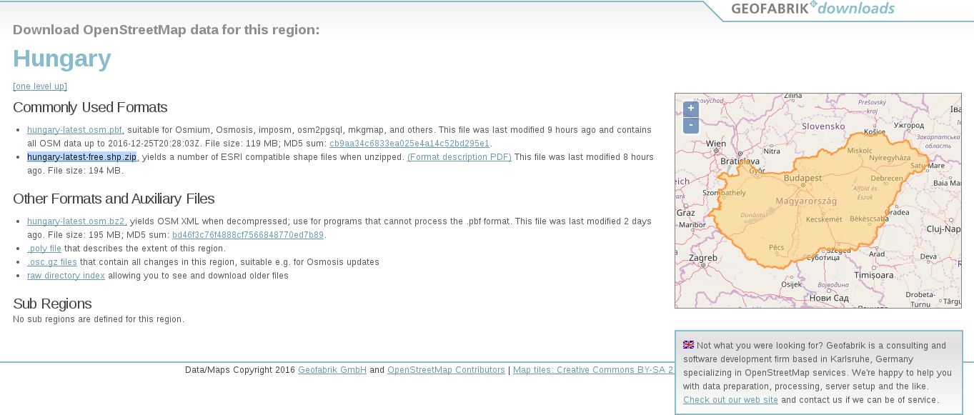
Due to various reasons, open source shapefiles are only exported by Geofabrik for small areas. We have to narrow down our search by clicking on links until the shapefile format (.shp.zip) is available. This means country-level extracts for smaller countries and regional extracts for larger or denser ones. The term dense refers to the amount of data stored in the OSM database for a given country. Let's download the shapefile for the smallest region enveloping our study area:
OpenStreetMap data is licensed under ODbL, an open source license, and therefore gives the four basic freedoms. However, it has two important conditions. The first one is obligatory attribution, while the second one is a share-alike condition. If we use OpenStreetMap data in our work, we must share the OSM part under an ODbL-compatible open source license.
ODbL differentiates three kind of products: collective database, derived database, and produced work. If we create a collective database (a database which has an OSM part), the share-alike policy only applies on the OSM part. If we create a derived database (make modifications to the OSM database), we must make the whole thing open source. If we create a map, a game, or any other work based on the OSM database, we can use any license we would like to. However, if we modify the OSM database during the process, we must make the modifications open source.
Note
If the license would only have these rules, it could be abused in infinitesimal ways. Therefore, the full license contains a lot more details and some clauses to avoid abuses. You can learn more about ODbL at https://wiki.osmfoundation.org/wiki/Licence.