
In computer vision and image processing, color space refers to a specific way of organizing colors. A color space is actually a combination of two things, a color model and a mapping function. The reason we want color models is because it helps us in representing pixel values using tuples. The mapping function maps the color model to the set of all possible colors that can be represented.
There are many different color spaces that are useful. Some of the more popular color spaces are RGB, YUV, HSV, Lab, and so on. Different color spaces provide different advantages. We just need to pick the color space that's right for the given problem. Let's take a couple of color spaces and see what information they provide:
- RGB: Probably the most popular color space. It stands for Red, Green, and Blue. In this color space, each color is represented as a weighted combination of red, green, and blue. So every pixel value is represented as a tuple of three numbers corresponding to red, green, and blue. Each value ranges between 0 and 255.
- YUV: Even though RGB is good for many purposes, it tends to be very limited for many real-life applications. People started thinking about different methods to separate the intensity information from the color information. Hence, they came up with the YUV color space. Y refers to the luminance or intensity, and U/V channels represent color information. This works well in many applications because the human visual system perceives intensity information very differently from color information.
- HSV: As it turned out, even YUV was still not good enough for some applications. So people started thinking about how humans perceive color, and they came up with the HSV color space. HSV stands for Hue, Saturation, and Value. This is a cylindrical system where we separate three of the most primary properties of colors and represent them using different channels. This is closely related to how the human visual system understands color. This gives us a lot of flexibility as to how we can handle images.
Considering all the color spaces, there are around 190 conversion options available in OpenCV. If you want to see a list of all available flags, go to the Python shell and type the following:
import cv2
print([x for x in dir(cv2) if x.startswith('COLOR_')])
You will see a list of options available in OpenCV for converting from one color space to another. We can pretty much convert any color space to any other color space. Let's see how we can convert a color image to a grayscale image:
import cv2
img = cv2.imread('./images/input.jpg', cv2.IMREAD_COLOR)
gray_img = cv2.cvtColor(img, cv2.COLOR_RGB2GRAY)
cv2.imshow('Grayscale image', gray_img)
cv2.waitKey()You can convert to YUV by using the following flag:
yuv_img = cv2.cvtColor(img, cv2.COLOR_BGR2YUV)
The image will look something like the following one:
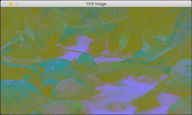
This may look like a deteriorated version of the original image, but it's not. Let's separate out the three channels:
# Alternative 1
y,u,v = cv2.split(yuv_img)
cv2.imshow('Y channel', y)
cv2.imshow('U channel', u)
cv2.imshow('V channel', v)
cv2.waitKey()
# Alternative 2 (Faster)
cv2.imshow('Y channel', yuv_img[:, :, 0])
cv2.imshow('U channel', yuv_img[:, :, 1])
cv2.imshow('V channel', yuv_img[:, :, 2])
cv2.waitKey()Since yuv_img is a NumPy (which provides dimensional selection operators), we can separate out the three channels by slicing it. If you look at yuv_img.shape, you will see that it is a 3D array. So once you run the preceding piece of code, you will see three different images. Following is the Ychannel:
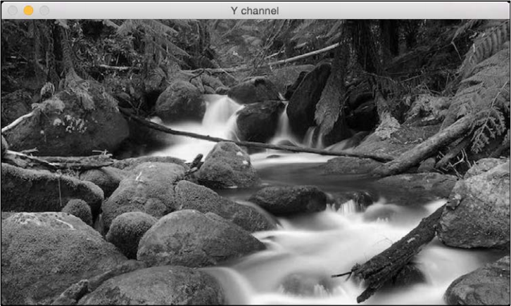
The channel is basically the grayscale image. Next is the U channel:
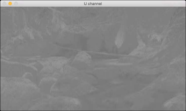
And lastly, the V channel:
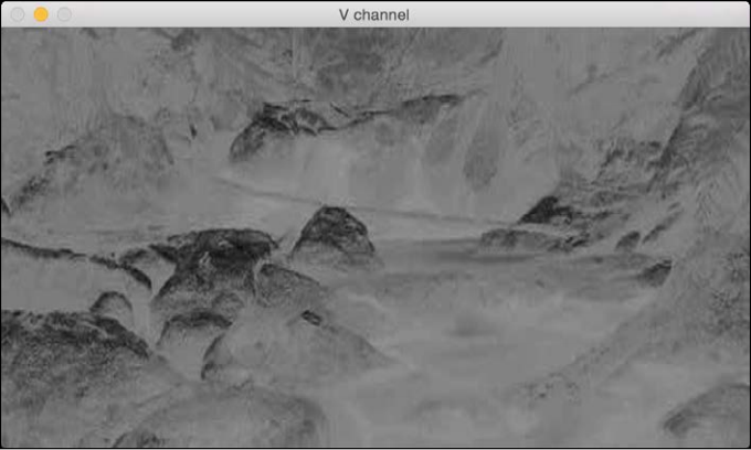
As we can see here, the channel is the same as the grayscale image. It represents the intensity values, and channels represent the color information.
Now we are going to read an image, split it into separate channels, and merge them to see how different effects can be obtained out of different combinations:
img = cv2.imread('./images/input.jpg', cv2.IMREAD_COLOR)
g,b,r = cv2.split(img)
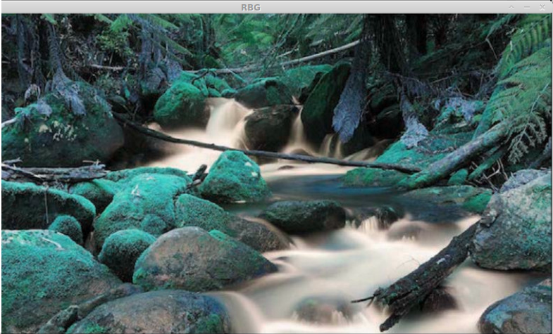
gbr_img = cv2.merge((g,b,r))
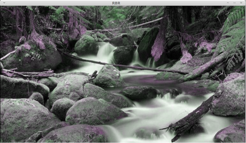
rbr_img = cv2.merge((r,b,r))
cv2.imshow('Original', img)
cv2.imshow('GRB', gbr_img)
cv2.imshow('RBR', rbr_img)
cv2.waitKey()Here we can see how channels can be recombined to obtain different color intensities:
In this one, the red channel is used twice so the reds are more intense:
This should give you a basic idea of how to convert between color spaces. You can play around with more color spaces to see what the images look like. We will discuss the relevant color spaces as and when we encounter them during subsequent chapters.