
In this section, we will discuss the various generalized geometrical transformations of 2D images. We have been using the function warpAffine quite a bit over the last couple of sections, it's about time we understood what's happening underneath.
Before talking about affine transformations, let's learn what Euclidean transformations are. Euclidean transformations are a type of geometric transformation that preserve length and angle measures. If we take a geometric shape and apply Euclidean transformation to it, the shape will remain unchanged. It might look rotated, shifted, and so on, but the basic structure will not change. So technically, lines will remain lines, planes will remain planes, squares will remain squares, and circles will remain circles.
Coming back to affine transformations, we can say that they are generalizations of Euclidean transformations. Under the realm of affine transformations, lines will remain lines, but squares might become rectangles or parallelograms. Basically, affine transformations don't preserve lengths and angles.
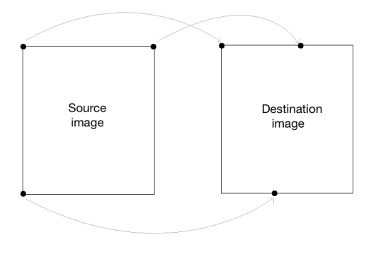
In order to build a general affine transformation matrix, we need to define the control points. Once we have these control points, we need to decide where we want them to be mapped. In this particular situation, all we need are three points in the source image, and three points in the output image. Let's see how we can convert an image into a parallelogram-like image:
import cv2
import numpy as np
img = cv2.imread('images/input.jpg')
rows, cols = img.shape[:2]
src_points = np.float32([[0,0], [cols-1,0], [0,rows-1]])
dst_points = np.float32([[0,0], [int(0.6*(cols-1)),0], [int(0.4*(cols-1)),rows-1]])
affine_matrix = cv2.getAffineTransform(src_points, dst_points)
img_output = cv2.warpAffine(img, affine_matrix, (cols,rows))
cv2.imshow('Input', img)
cv2.imshow('Output', img_output)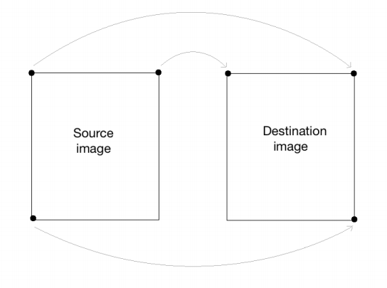
cv2.waitKey()As we discussed earlier, we are defining control points. We just need three points to get the affine transformation matrix. We want the three points in src_points to be mapped to the corresponding points in dst_points. We are mapping the points as shown in the following image:
To get the transformation matrix, we have a function called in OpenCV. Once we have the affine transformation matrix, we use the function to apply this matrix to the input image.
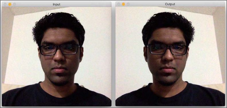
Following is the input image:

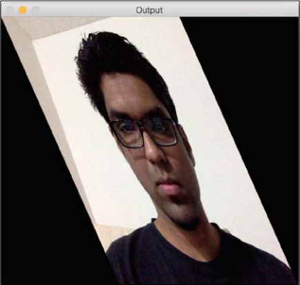
If you run the preceding code, the output will look something like this:
We can also get the mirror image of the input image. We just need to change the control points in the following way:
src_points = np.float32([[0,0], [cols-1,0], [0,rows-1]])
dst_points = np.float32([[cols-1,0], [0,0], [cols-1,rows-1]])
Here, the mapping looks something like this:
If you replace the corresponding lines in our affine transformation code with these two lines, you will get the following result: