
Now that we have learned the importance of Python, we will start by exploring various basic data structures in Python. We will learn techniques to handle data. This is invaluable for a data practitioner.
We can issue the following command to start a new Jupyter server by typing the following in to the Command Prompt window:
docker run -p 8888:8888 -v 'pwd':/notebooks -it rcshubhadeep/packt-data-wrangling-base:latest ipython
This will start a jupyter server and you can visit it at http://localhost:8888 and use the passcode dw_4_all to access the main interface.
Lists are fundamental Python data structures that have continuous memory locations, can host different data types, and can be accessed by the index.
We will start with a list and list comprehension. We will generate a list of numbers, and then examine which ones among them are even. We will sort, reverse, and check for duplicates. We will also see how many different ways we can access the list elements, iterating over them and checking the membership of an element.
The following is an example of a simple list:
list_example = [51, 27, 34, 46, 90, 45, -19]
The following is also an example of a list:
list_example2 = [15, "Yellow car", True, 9.456, [12, "Hello"]]
As you can see, a list can contain any number of the allowed datatype, such as int, float, string, and Boolean, and a list can also be a mix of different data types (including nested lists).
If you are coming from a strongly typed language, such as C, C++, or Java, then this will probably be strange as you are not allowed to mix different kinds of data types in a single array in those languages. Lists are somewhat like arrays, in the sense that they are both based on continuous memory locations and can be accessed using indexes. But the power of Python lists come from the fact that they can host different data types and you are allowed to manipulate the data.
In the following exercise, we will be creating a list and then observing the different ways of accessing the elements:
Define a list called list_1 with four integer members, using the following command:
list_1 = [34, 12, 89, 1]
The indices will be automatically assigned, as follows:
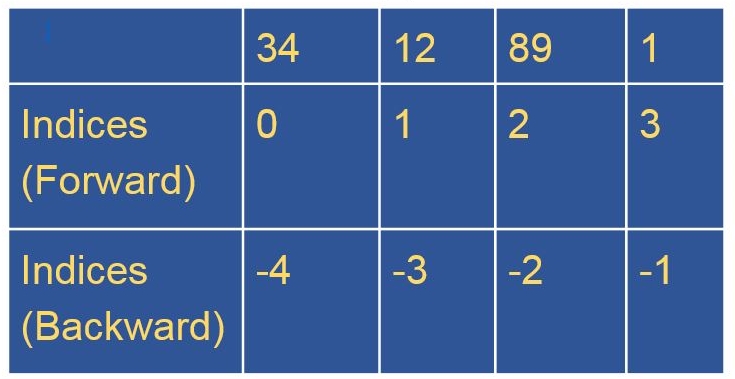
Figure 1.3: List showing the forward and backward indices
Access the first element from list_1 using its forward index:
list_1[0] #34
Access the last element from list_1 using its forward index:
list_1[3] #1
Access the last element from list_1 using the len function:
list_1[len(list_1) - 1] #1
The len function in Python returns the length of the specified list.
Access the last element from list_1 using its backward index:
list_1[-1] #1
Access the first three elements from list_1 using forward indices:
list_1[1:3] # [12, 89]
This is also called list slicing, as it returns a smaller list from the original list by extracting only, a part of it. To slice a list, we need two integers. The first integer will denote the start of the slice and the second integer will denote the end-1 element.
Access the last two elements from list_1 by slicing:
list_1[-2:] # [89, 1]
Access the first two elements using backward indices:
list_1[:-2] # [34, 12]
When we leave one side of the colon (:) blank, we are basically telling Python either to go until the end or start from the beginning of the list. It will automatically apply the rule of list slices that we just learned.
Reverse the elements in the string:
list_1[-1::-1] # [1, 89, 12, 34]
We are going to examine various ways of generating a list:
Create a list using the append method:
list_1 = []
for x in range(0, 10):
    list_1.append(x)
list_1
The output will be as follows:
[0, 1, 2, 3, 4, 5, 6, 7, 8, 9]
Here, we started by declaring an empty list and then we used a for loop to append values to it. The append method is a method that's given to us by the Python list data type.
Generate a list using the following command:
list_2 = [x for x in range(0, 100)]
list_2
The partial output is as follows:
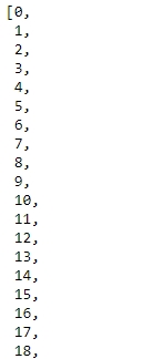
Figure 1.4: List comprehension
This is list comprehension, which is a very powerful tool that we need to master. The power of list comprehension comes from the fact that we can use conditionals inside the comprehension itself.
Use a while loop to iterate over a list to understand the difference between a while loop and a for loop:
i = 0
while i < len(list_1) :
    print(list_1[i])
    i += 1
The partial output will be as follows:

Figure 1.5: Output showing the contents of list_1 using a while loop
Create list_3 with numbers that are divisible by 5:
list_3 = [x for x in range(0, 100) if x % 5 == 0]
list_3
The output will be a list of numbers up to 100 in increments of 5:
[0, 5, 10, 15, 20, 25, 30, 35, 40, 45, 50, 55, 60, 65, 70, 75, 80, 85, 90, 95]
Generate a list by adding the two lists:
list_1 = [1, 4, 56, -1]
list_2 = [1, 39, 245, -23, 0, 45]
list_3 = list_1 + list_2
list_3
The output is as follows:
[1, 4, 56, -1, 1, 39, 245, -23, 0, 45]
Extend a string using the extend keyword:
list_1.extend(list_2)
list_1
The partial output is as follows:

Figure 1.6: Contents of list_1
The second operation changes the original list (list_1) and appends all the elements of list_2 to it. So, be careful when using it.
We are going to iterate over a list and test whether a certain value exists in it:
Iterate over a list:
list_1 = [x for x in range(0, 100)]
for i in range(0, len(list_1)):
    print(list_1[i])
The output is as follows:

Figure 1.7: Section of list_1
However, it is not very Pythonic. Being Pythonic is to follow and conform to a set of best practices and conventions that have been created over the years by thousands of very able developers, which in this case means to use the in keyword, because Python does not have index initialization, bounds checking, or index incrementing, unlike traditional languages. The Pythonic way of iterating over a list is as follows:
for i in list_1:
    print(i)
The output is as follows:

Figure 1.8: A section of list_1
Notice that, in the second method, we do not need a counter anymore to access the list index; instead, Python's in operator gives us the element at the i th position directly.
Check whether the integers 25 and -45 are in the list using the in operator:
25 in list_1
The output is True.
-45 in list_1
The output is False.
We generated a list called list_1 in the previous exercise. We are going to sort it now:
Note
The difference between the sort function and the reverse function is the fact that we can use sort with custom sorting functions to do custom sorting, whereas we can only use reverse to reverse a list. Here also, both the functions work in-place, so be aware of this while using them.
As the list was originally a list of numbers from 0 to 99, we will sort it in the reverse direction. To do that, we will use the sort method with reverse=True:
list_1.sort(reverse=True)
list_1
The partial output is as follows:

Figure 1.9: Section of output showing the reversed list
We can use the reverse method directly to achieve this result:
list_1.reverse()
list_1
The output is as follows:

Figure 1.10: Section of output after reversing the string
In this exercise, we will be generating a list with random numbers:
Import the random library:
import random
Use the randint function to generate random integers and add them to a list:
list_1 = [random.randint(0, 30) for x in range (0, 100)]
Print the list using print(list_1). Note that there will be duplicate values in list_1:
list_1
The sample output is as follows:

Figure 1.11: Section of the sample output for list_1
There are many ways to get a list of unique numbers, and while you may be able to write a few lines of code using a for loop and another list (you should actually try doing it!), let's see how we can do this without a for loop and with a single line of code. This will bring us to the next data structure, sets.
In this activity, we will generate a list of random numbers and then generate another list from the first one, which only contains numbers that are divisible by three. Repeat the experiment three times. Then, we will calculate the average difference of length between the two lists.
These are the steps for completing this activity:
Create a list of 100 random numbers.
Create a new list from this random list, with numbers that are divisible by 3.
Calculate the length of these two lists and store the difference in a new variable.
Using a loop, perform steps 2 and 3 and find the difference variable three times.
Find the arithmetic mean of these three difference values.
A set, mathematically speaking, is just a collection of well-defined distinct objects. Python gives us a straightforward way to deal with them using its set datatype.
With the last list that we generated, we are going to revisit the problem of getting rid of duplicates from it. We can achieve that with the following line of code:
list_12 = list(set(list_1))
If we print this, we will see that it only contains unique numbers. We used the set data type to turn the first list into a set, thus getting rid of all duplicate elements, and then we used the list function on it to turn it into a list from a set once more:
list_12
The output will be as follows:

Figure 1.12: Section of output for list_21
This is what a union between two sets looks like:
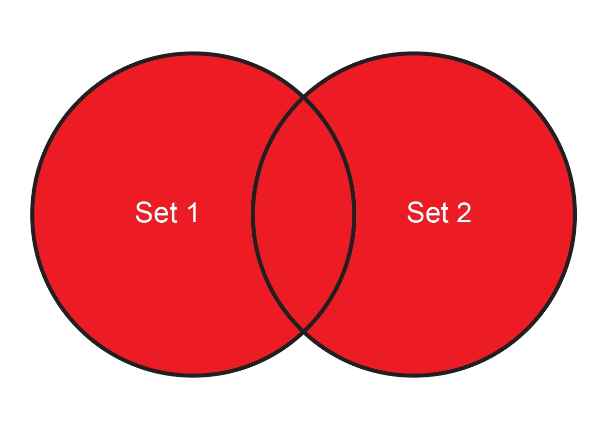
Figure 1.13: Venn diagram showing the union of two sets
This simply means take everything from both sets but take the common elements only once.
We can create this using the following code:
set1 = {"Apple", "Orange", "Banana"}
set2 = {"Pear", "Peach", "Mango", "Banana"}
To find the union of the two sets, the following instructions should be used:
set1 | set2
The output would be as follows:
{'Apple', 'Banana', 'Mango', 'Orange', 'Peach', 'Pear'}Notice that the common element, Banana, appears only once in the resulting set. The common elements between two sets can be identified by obtaining the intersection of the two sets, as follows:
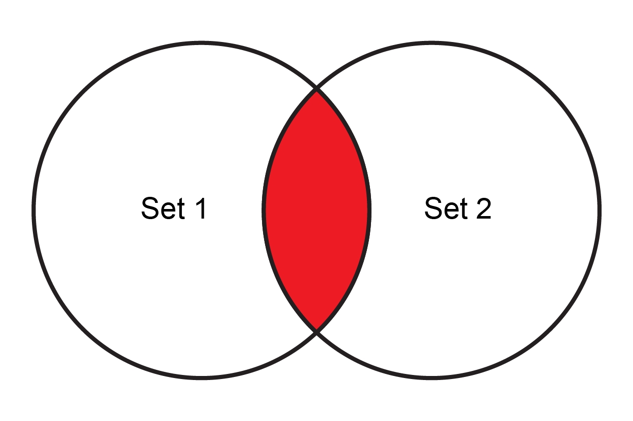
Figure 1.14: Venn diagram showing the intersection of two sets
We get the intersection of two sets in Python as follows:
set1 & set2
This will give us a set with only one element. The output is as follows:
{'Banana'}Note
You can also calculate the difference between sets (also known as complements). To find out more, refer to this link: https://docs.python.org/3/tutorial/datastructures.html#sets.
You can create a null set by creating a set containing no elements. You can do this by using the following code:
null_set_1 = set({})
null_set_1
The output is as follows:
set()
However, to create a dictionary, use the following command:
null_set_2 = {}
null_set_2
The output is as follows:
{}We are going to learn about this in detail in the next topic.
A dictionary is like a list, which means it is a collection of several elements. However, with the dictionary, it is a collection of key-value pairs, where the key can be anything that can be hashed. Generally, we use numbers or strings as keys.
To create a dictionary, use the following code:
dict_1 = {"key1": "value1", "key2": "value2"}
dict_1
The output is as follows:
{'key1': 'value1', 'key2': 'value2'}This is also a valid dictionary:
dict_2 = {"key1": 1, "key2": ["list_element1", 34], "key3": "value3",
          "key4": {"subkey1": "v1"}, "key5": 4.5}
dict_2
The output is as follows:
{'key1': 1,
 'key2': ['list_element1', 34],
 'key3': 'value3',
 'key4': {'subkey1': 'v1'},
 'key5': 4.5}
The keys must be unique in a dictionary.
In this exercise, we are going to access and set values in a dictionary:
Access a particular key in a dictionary:
dict_2["key2"]
This will return the value associated with it as follows:
['list_element1', 34]
Assign a new value to the key:
dict_2["key2"] = "My new value"
Define a blank dictionary and then use the key notation to assign values to it:
dict_3 = {}  # Not a null set. It is a dict
dict_3["key1"] = "Value1"
dict_3
The output is as follows:
{'key1': 'Value1'}
In this exercise, we are going to iterate over a dictionary:
Create dict_1:
dict_1 = {"key1": 1, "key2": ["list_element1", 34], "key3": "value3", "key4": {"subkey1": "v1"}, "key5": 4.5}Use the looping variables k and v:
for k, v in dict_1.items():
    print("{} - {}".format(k, v))
The output is as follows:
key1 - 1
key2 - ['list_element1', 34]
key3 - value3
key4 - {'subkey1': 'v1'}
key5 - 4.5
We will use the fact that dictionary keys cannot be duplicated to generate the unique valued list:
First, generate a random list with duplicate values:
list_1 = [random.randint(0, 30) for x in range (0, 100)]
Create a unique valued list from list_1:
list(dict.fromkeys(list_1).keys())
The sample output is as follows:

Figure 1.15: Output showing the unique valued list
Here, we have used two useful functions on the dict data type in Python, fromkeys and keys. fromkeys creates a dict where the keys come from the iterable (in this case, which is a list), values default to None, and keys give us the keys of a dict.
In this exercise, we are going to delete a value from a dict:
Create list_1 with five elements:
dict_1 = {"key1": 1, "key2": ["list_element1", 34], "key3": "value3",
          "key4": {"subkey1": "v1"}, "key5": 4.5}
dict_1
The output is as follows:
{'key1': 1,
 'key2': ['list_element', 34],
 'key3': 'value3',
 'key4': {'subkey1': 'v1'},
 'key5': 4.5}
We will use the del function and specify the element:
del dict_1["key2"]
The output is as follows:
{'key3': 'value3', 'key4': {'subkey1': 'v1'}, 'key5': 4.5}
In this final exercise on dict, we will go over a less used comprehension than the list one: dictionary comprehension. We will also examine two other ways to create a dict, which will be useful in the future.
A dictionary comprehension works exactly the same way as the list one, but we need to specify both the keys and values:
Generate a dict that has 0 to 9 as the keys and the square of the key as the values:
list_1 = [x for x in range(0, 10)]
dict_1 = {x : x**2 for x in list_1}
dict_1
The output is as follows:
{0: 0, 1: 1, 2: 4, 3: 9, 4: 16, 5: 25, 6: 36, 7: 49, 8: 64, 9: 81}Can you generate a dict using dict comprehension where the keys are from 0 to 9 and the values are the square root of the keys? This time, we won't use a list.
Generate a dictionary using the dict function:
dict_2 = dict([('Tom', 100), ('Dick', 200), ('Harry', 300)])
dict_2
The output is as follows:
{'Tom': 100, 'Dick': 200, 'Harry': 300}You can also generate dictionary using the dict function, as follows:
dict_3 = dict(Tom=100, Dick=200, Harry=300)
dict_3
The output is as follows:
{'Tom': 100, 'Dick': 200, 'Harry': 300}It is pretty versatile. So, both the preceding commands will generate valid dictionaries.
The strange looking pair of values that we had just noticed ('Harry', 300) is called a tuple. This is another important fundamental data type in Python. We will learn about tuples in the next topic.
A tuple is another data type in Python. It is sequential in nature and similar to lists.
A tuple consists of values separated by commas, as follows:
tuple_1 = 24, 42, 2.3456, "Hello"
Notice that, unlike lists, we did not open and close square brackets here.
This is how we create an empty tuple:
tuple_1 = ()
And this is how we create a tuple with only one value:
tuple_1 = "Hello",
Notice the trailing comma here.
We can nest tuples, similar to list and dicts, as follows:
tuple_1 = "hello", "there"
tuple_12 = tuple_1, 45, "Sam"
One special thing about tuples is the fact that they are an immutable data type. So, once created, we cannot change their values. We can just access them, as follows:
tuple_1 = "Hello", "World!"
tuple_1[1] = "Universe!"
The last line of code will result in a TypeError as a tuple does not allow modification.
This makes the use case for tuples a bit different than lists, although they look and behave very similarly in a few aspects.
The term unpacking a tuple simply means to get the values contained in the tuple in different variables:
tuple_1 = "Hello", "World"
hello, world = tuple_1
print(hello)
print(world)
The output is as follows:
Hello
World
Of course, as soon as we do that, we can modify the values contained in those variables.
Create a tuple to demonstrate how tuples are immutable. Unpack it to read all elements, as follows:
tupleE = "1", "3", "5"
tupleE
The output is as follows:
('1', '3', '5')Try to override a variable from the tupleE tuple:
tupleE[1] = "5"
This step will result in TypeError as the tuple does not allow modification.
Try to assign a series to the tupleE tuple:
1, 3, 5 = tupleE
Print the output:
print(1)
print(3)
The output is as follows:
1
3
We have mainly seen two different types of data so far. One is represented by numbers; another is represented by textual data. Whereas numbers have their own tricks, which we will see later, it is time to look into textual data in a bit more detail.
In the final section of this section, we will learn about strings. Strings in Python are similar to any other programming language.
This is a string:
string1 = 'Hello World!'
A string can also be declared in this manner:
string2 = "Hello World 2!"
You can use single quotes and double quotes to define a string.
Strings in Python behave similar to lists, apart from one big caveat. Strings are immutable, whereas lists are mutable data structures:
Create a string called str_1:
str_1 = "Hello World!"
Access the elements of the string by specifying the location of the element, like we did in lists.
Access the first member of the string:
str_1[0]
The output is as follows:
'H'
Access the fourth member of the string:
str_1[4]
The output is as follows:
'o'
Access the last member of the string:
str_1[len(str_1) - 1]
The output is as follows:
'!'
Access the last member of the string:
str_1[-1]
The output is as follows:
'!'
Each of the preceding operations will give you the character at the specific index.
Just like lists, we can slice strings:
Create a string, str_1:
str_1 = "Hello World! I am learning data wrangling"
Specify the slicing values and slice the string:
str_1[2:10]
The output is this:
'llo Worl'
Slice a string by skipping a slice value:
str_1[-31:]
The output is as follows:
'd! I am learning data wrangling'
Use negative numbers to slice the string:
str_1[-10:-5]
The output is as follows:
' wran'
To find out the length of a string, we simply use the len function:
str_1 = "Hello World! I am learning data wrangling"
len(str_1)
The length of the string is 41. To convert a string's case, we can use the lower and upper methods:
str_1 = "A COMPLETE UPPER CASE STRING"
str_1.lower()
str_1.upper()
The output is as follows:
'A COMPLETE UPPER CASE STRING'
To search for a string within a string, we can use the find method:
str_1 = "A complicated string looks like this"
str_1.find("complicated")
str_1.find("hello")# This will return -1
The output is -1. Can you figure out whether the find method is case-sensitive or not? Also, what do you think the find method returns when it actually finds the string?
To replace one string with another, we have the replace method. Since we know that a string is an immutable data structure, replace actually returns a new string instead of replacing and returning the actual one:
str_1 = "A complicated string looks like this"
str_1.replace("complicated", "simple")
The output is as follows:
'A simple string looks like this'
You should look up string methods in the standard documentation of Python 3 to discover more about these methods.
These two string methods need separate introductions, as they enable you to convert a string into a list and vice versa:
Create a string and convert it to a list using the split method:
str_1 = "Name, Age, Sex, Address"
list_1 = str_1.split(",")
list_1
The preceding code will give you a list similar to the following:
['Name', ' Age', ' Sex', ' Address']
Combine this list into another string using the join method:
" | ".join(list_1)
This code will give you a string like this:
'Name | Age | Sex | Address'
With these, we are at the end of our second topic of this chapter. We now have the motivation to learn data wrangling and have a solid introduction to the fundamentals of data structures using Python. There is more to this topic, which will be covered in a future chapters.
We have designed an activity for you so that you can practice all the skills you just learned. This small activity should take around 30 to 45 minutes to finish.
This section will ensure that you have understood the various basic data structures and their manipulation. We will do that by going through an activity that has been designed specifically for this purpose.
In this activity, we will do the following:
Get multiline text and save it in a Python variable
Get rid of all new lines in it using string methods
Get all the unique words and their occurrences from the string
Repeat the step to find all unique words and occurrences, without considering case sensitivity
Note
For the sake of simplicity for this activity, the original text (which can be found at https://www.gutenberg.org/files/1342/1342-h/1342-h.htm) has been pre-processed a bit.
These are the steps to guide you through solving this activity:
Create a mutliline_text variable by copying the text from the first chapter of Pride and Prejudice.
Note
The first chapter of Pride and Prejudice by Jane Austen has been made available on the GitHub repository at https://github.com/TrainingByPackt/Data-Wrangling-with-Python/blob/master/Chapter01/Activity02/.
Find the type and length of the multiline_text string using the commands type and len.
Remove all new lines and symbols using the replace function.
Find all of the words in multiline_text using the split function.
Create a list from this list that will contain only the unique words.
Count the number of times the unique word has appeared in the list using the key and value in dict.
Find the top 25 words from the unique words that you have found using the slice function.
You just created, step by step, a unique word counter using all the neat tricks that you learned about in this chapter.