
R objects can be grouped into two categories:
Atomic vectors, Matrices, or Arrays are data structures that are used to store homogenous data, while Lists and Data frames are typically used to store heterogeneous data. R objects can also be organized based on the number of dimensions they contain. For example, atomic vectors and lists are one-dimensional objects, whereas matrices and data frames are two-dimensional objects. Arrays, however, are objects that can have any number of dimensions. Unlike other programming languages such as Perl, R does not have scalar or zero-dimensional objects. All single numbers and strings are stored in vectors of length one.
Vectors are the basic data structure in R and include atomic vectors and lists. Atomic vectors are flat and can be logical, numeric (double), integer, character, complex, or raw. To create a vector, we use the c() function, which means combine elements into a vector:
> x <- c(1, 2, 3)
To create an integer vector, add the number followed by L, as follows:
> integer_vector <- c(1L, 2L, 12L, 29L)
> integer_vector
[1]  1  2 12 29
To create a logical vector, add TRUE (T) and FALSE (F), as follows:.
> logical_vector <- c(T, TRUE, F, FALSE)
> logical_vector
[1]  TRUE  TRUE FALSE FALSE
Tip
Downloading the example code
You can download the example code files from your account at http://www.packtpub.com for all the Packt Publishing books you have purchased. If you purchased this book elsewhere, you can visit http://www.packtpub.com/support and register to have the files e-mailed directly to you.
To create a vector containing strings, simply add the words/phrases in double quotes:
> character_vector <- c("Apple", "Pear", "Red", "Green", "These are my favorite fruits and colors")
> character_vector
[1] "Apple"
[2] "Pear"
[3] "Red"
[4] "Green"
[5] "These are my favorite fruits and colors"
> numeric_vector <- c(1, 3.4, 5, 10)
> numeric_vector
[1]  1.0  3.4  5.0 10.0
R also includes functions that allow you to create vectors containing repetitive elements with rep() or a sequence of numbers with seq():
> seq(1, 12, by=3)
[1]  1  4  7 10
> seq(1, 12) #note the default parameter for by is 1
 [1]  1  2  3  4  5  6  7  8  9 10 11 12
Instead of using the seq() function, you can also use a colon, :, to indicate that you would like numbers 1 to 12 to be stored as a vector, as shown in the following example:
> y <- 1:12
> y
 [1]  1  2  3  4  5  6  7  8  9 10 11 12
> z <- c(1:3, y)
> z
 [1]  1  2  3  1  2  3  4  5  6  7  8  9 10 11 12
To replicate elements of a vector, you can simply use the rep() function, as follows:
> x <- rep(3, 14)
> x
 [1] 3 3 3 3 3 3 3 3 3 3 3 3 3 3
You can also replicate complex patterns as follows:
> rep(seq(1, 4), 3)
 [1] 1 2 3 4 1 2 3 4 1 2 3 4
Atomic vectors can only be of one type so if you mix numbers and strings, your vector will be coerced into the most flexible type. The most to the least flexible vector types are Character, numeric, integer, and logical, as shown in the following diagram:
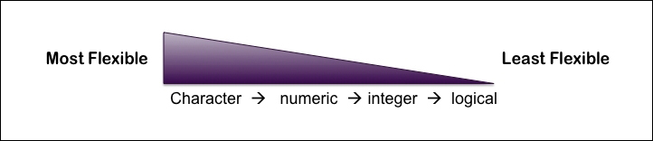
This means that if you mix numbers with strings, your vector will be coerced into a character vector, which is the most flexible type of the two. In the following paragraph, there are two different examples showing this coercion in practice. The first example shows that when a character and numeric vector are combined, the class of this new object becomes a character vector because a character vector is more flexible than a numeric vector. Similarly, in the second example, we see that the class of the new object x is numeric because a numeric vector is more flexible than an integer vector. The two examples are as follows:
Example 1:
> mixed_vector <- c(character_vector, numeric_vector)
> mixed_vector
[1] "Apple"
[2] "Pear"
[3] "Red"
[4] "Green"
[5] "These are my favorite fruits and colors"
[6] "1"
[7] "3.4"
[8] "5"
[9] "10"
> class(mixed_vector)
[1] "character"
Example 2:
> x <- c(integer_vector, numeric_vector)
> x
[1]  1.0  2.0 12.0 29.0  1.0  3.4  5.0 10.0
> class(x)
[1] "numeric"
At times, you may create a group of objects and forget its name or content. R allows you to quickly retrieve this information using the ls() function, which returns a vector of the names of the objects specified in the current workspace or environment.
> ls()
[1] "a"  "A"  "b"  "B"  "C"  "character_vector"  "influence.1"
[8] "influence.1.2"  "influence.2"  "integer_vector"  "logical_vector"  "M"  "mixed_vector"  "N"
[15] "numeric_vector"  "P"  "Q"  "second.degree.mat"  "small.network"  "social.network.mat" "x"
[22] "y"
At first glance, the workspace or environment is the space where you store all the objects you create. More formally, it consists of a frame or collection of named objects, and a pointer to an enclosing environment. When we created the variable x, we added it to the global environment, but we could have also created a novel environment and stored it there. For example, let's create a numeric vector y and store it in a new environment called environB. To create a new environment in R, we use the new.env() function as follows:
> environB <- new.env()
> ls(environB)
character(0)
As you can see, there are no objects stored in this environment yet because we haven't created any. Now let's create a numeric vector y and assign it to environB using the assign() function:
> assign("y", c(1, 5, 9), envir=environB)
> ls(environB)
[1] "y"
Alternatively, we could use the $ sign to assign a new variable to environB as follows:
> environB$z <- "purple"
> ls(environB)
[1] "y" "z"
To see what we stored in y and z, we can use the get() function or the $ sign as follows:
> get('y', envir=environB)
[1] 1 5 9
> get('z', envir=environB)
[1] "purple"
> environB$y
[1] 1 5 9
You can also retrieve additional information on the objects stored in your environment using the str() function. This function allows you to inspect the internal structure of the object and print a preview of its contents as follows:
> str(character_vector)
 chr [1:5] "Apple" "Pear" "Red" "Green" ...
> str(integer_vector)
 int [1:4] 1 2 12 29
> str(logical_vector)
 logi [1:4] TRUE TRUE FALSE FALSE
To know how many elements are present in our vector, you can use the length() function as follows:
> length(integer_vector)
[1] 4
Finally, to extract elements from a vector, you can use the position (or index) of the element in square brackets as follows:
> character_vector[5]
[1] "These are my favorite fruits and colors"
> numeric_vector[2]
[1] 3.4
> x <- c(1, 4, 6)
> x[2]
[1] 4
Basic mathematical operations can be performed on numeric and integer vectors similar to those you perform on a calculator. The arithmetic operations used are given in the following table:
|
Arithmetic operators |
|---|
|
|
|
|
|
|
|
|
|
|
|
|
|
|
|
|
|
|
For example, if we multiply a vector by 2, all the elements of the vector will be multiplied by 2. Let's take a look at the following example:
> x <- c(1, 3, 5, 10)
> x * 2
[1]  2  6 10 20
You can also add vectors to each other, in which case the computation will be performed element-wise as follows:
> x <- c(1, 3, 5, 10)
> y <- c(13, 15, 17, 22)
> x + y
[1] 14 18 22 32
If the vectors are of different lengths, the shorter vector will be extended to match the length of the longer vector by recycling its elements starting from the first element. However, you will also get a warning message from R in case you did not intend to add vectors of differing length, as follows:
> x
[1]  1  3  5 10
> z <- c(1,3, 4, 6, 10)
> x + z #1 was recycled to complete the operation.
[1]  2  6  9 16 11
Warning message:
In x + z : longer object length is not a multiple of shorter object length
In addition to this, the standard operators also have %%, which indicates x mod y, and %/%, which indicates integer division as follows:
> x %% 2
[1] 1 1 1 0
> x %/% 5
[1] 0 0 1 2
Unlike atomic vectors, lists can contain different types of elements including lists. To create a list, you use the list() function as follows:
> simple_list <- list(1:4, rep(3, 5), "cat")
> str(simple_list)
List of 3
 $ : int [1:4] 1 2 3 4
 $ : num [1:5] 3 3 3 3 3
 $ : chr "cat"
> other_list <- list(1:4, "I prefer pears", logical_vector, x, simple_list)
> str(other_list)
List of 5
 $ : int [1:4] 1 2 3 4
 $ : chr "I prefer pears"
 $ : logi [1:4] TRUE TRUE FALSE FALSE
 $ : num [1:3] 1 4 6
 $ :List of 3
  ..$ : int [1:4] 1 2 3 4
  ..$ : num [1:5] 3 3 3 3 3
  ..$ : chr "cat"
If you use the c() function to combine lists and atomic vectors, c() will coerce the vectors to lists of length one before proceeding. Let's go through a detailed example in R:
> new_list <- c(list(1, 2, simple_list), c(3, 4), seq(5, 6))
Now, let's take a look at the output of the list we just created by entering new_list in R:
> new_list
[[1]]
[1] 1

[[2]]
[1] 2

[[3]]
[[3]][[1]]
[1] 1 2 3 4

[[3]][[2]]
[1] 3 3 3 3 3

[[3]][[3]]
[1] "cat"


[[4]]
[1] 3

[[5]]
[1] 4

[[6]]
[1] 5

[[7]]
[1] 6
# Output truncated here
We can further inspect the new_list object that we just created using the str() function as follows:
> str(new_list)
List of 7
 $ : num 1
 $ : num 2
 $ :List of 3
  ..$ : int [1:4] 1 2 3 4
  ..$ : num [1:5] 3 3 3 3 3
  ..$ : chr "cat"
 $ : num 3
 $ : num 4
 $ : int 5
 $ : int 6
You can also coerce an atomic vector into a list using the as.list() function as follows:
> x_as_list <- as.list(x)
> str(x_as_list)
List of 4
 $ : num 1
 $ : num 3
 $ : num 5
 $ : num 10
To access different elements in your list, you can use the index position in square brackets [], as you would for a vector, or double square brackets [[]]. Let's take a look at the following example:
> simple_list
[[1]]
[1] 1 2 3 4
[[2]]
[1] 3 3 3 3 3
[[3]]
[1] "cat"
> simple_list[3]
[[1]]
[1] "cat"
As you will no doubt notice, by entering simple_list[3], R returns a list of the single element "cat" as follows:
> str(simple_list[3])
List of 1
 $ : chr "cat"
If we use the double square brackets, R will return the object type as we initially entered it. So, in this case, it would return a character vector for simple_list[[3]] and an integer vector for simple_list[[1]] as follows:
> str(simple_list[[3]])
 chr "cat"
> str(simple_list[[1]])
 int [1:4] 1 2 3 4
We can assign these elements to new objects as follows:
> animal <- simple_list[[3]]
> animal
[1] "cat"
> num_vector <- simple_list[[1]]
> num_vector
[1] 1 2 3 4
If you would like to access an element of an object in your list, you can use double square brackets [[ ]] followed by single square brackets [ ] as follows:
> simple_list[[1]][4]
[1] 4
> simple_list[1][4] #Note this format does not return the element
[[1]]
NULL
#Instead you would have to enter
> simple_list[1][[1]][4]
[1] 4
Objects in R can have additional attributes ascribed to objects that you can store with the attr() function, as shown in the following code:
> attr(x_as_list, "new_attribute") <- "This list contains the number of apples eaten for 3 different days"
> attr(x_as_list, "new_attribute")
[1] "This list contains the number of apples eaten for 3 different days"
> str(x_as_list)
List of 3
 $ : num 1
 $ : num 4
 $ : num 6
 - attr(*, "new_attribute")= chr "This list contains the number of apples eaten for 3 different days"
You can use the structure() function, as shown in the following code, to attach an attribute to an object you wish to return:
> structure(as.integer(1:7), added_attribute = "This vector contains integers.")
[1] 1 2 3 4 5 6 7
attr(,"added_attribute")
[1] "This vector contains integers."
In addition to attributes that you create with attr(), R also has built-in attributes ascribed to some of its functions, such as class(), dim(), and names(). The class() function tells us the class (type) of the object as follows:
> class(simple_list)
[1] "list"
The dim() function returns the dimension of higher-order objects such as matrices, data frames, and multidimensional arrays. The names() function allows you to give names to each element of your vector as follows:
> y <- c(first =1, second =2, third=4, fourth=4)
> y
 first second  third fourth
     1      2      4      4
You can use the names() attribute to add the names of each element to your vector as follows:
> element_names <- c("first", "second", "third", "fourth")
> y <- c(1, 2, 4, 4)
> names(y) <- element_names
> y
 first second  third fourth
     1      2      4      4
You can also modify the names of vector elements using the setNames() function as follows:
> setNames(y, c("alpha", "beta", "omega", "psi"))
alpha beta, omega   psi
    1     2     4     4
If you do not provide names for some of your vector elements, the names() function will return empty strings, <NA>, for the missing ones as follows:
> y <- setNames(y, c("alpha", "beta", "psi"))
> names(y)
[1] "alpha" "beta"  "psi"   NA
However, this does not mean that all vectors require names. In the event that you haven't provided any, names() will return NULL as follows:
> x <- 1:12
> x <- 1:12
> names(x)
NULL
You can remove names using the unname() function or by replacing the names with NULL:
> unname(y)
[1] 1 2 4 4
> names(y) <- NULL
> names(y)
NULL
When dealing with categorical data, R provides an alternative framework to store character data termed Factors. These are specialized vectors that contain predefined values referred to as Levels. For example, say you have data for "placebo" and "treatment" for four patients, you could store this information as factors instead of a character vector by using the following code:
> drug_response <- c("placebo", "treatment", "placebo", "treatment")
> drug_response <-  factor(drug_response)
> drug_response
[1] placebo   treatment placebo   treatment
Levels: placebo treatment
To check the integers used for each level, you can use the as.integer() function as follows:
> as.integer(drug_response)
[1] 1 2 1 2
Note that you can only adjust elements in a factor with data stored as levels. Say you wanted to change the drug_response attribute for the fourth patient from "treatment" to "refused treatment", you will get the following warning message:
> drug_response[4] <- "refused treatment"
Warning message:
In `[<-.factor`(`*tmp*`, 4, value = "refused treatment") :
  invalid factor level, NA generated
In order to correct this error, you need to first add a new level to the factor using the factor() function with the levels argument as follows:
> drug_response <- factor(drug_response, levels = c(levels(drug_response), "refused treatment"))
> drug_response[4] <- "refused treatment"
> drug_response
[1] placebo           treatment         placebo           refused treatment
Levels: placebo treatment refused treatment
> as.integer(drug_response)
[1] 1 2 1 3
Multidimensional arrays are created by adding dimensions to the atomic vector created. In computer science, an array is defined as a data structure consisting of elements identified by at least one array index. So, atomic vectors can be seen as one-dimensional arrays. However, as mentioned earlier, arrays can have more than one dimension. These arrays are termed multidimensional arrays. In R, you can create multidimensional arrays using the array() function. For example, you can create a three-dimensional array using the array() function and specify the dimensions with the dim argument using a vector. Let's create a three-dimensional array of coordinates where the maximal indices in each dimension is 2, 8, and 2 for the first, second, and third dimension, respectively:
> coordinates <- array(1:16, dim=c(2, 8, 2))
> coordinates
, , 1
     [,1] [,2] [,3] [,4] [,5] [,6] [,7] [,8]
[1,]    1    3    5    7    9   11   13   15
[2,]    2    4    6    8   10   12   14   16
, , 2
[,1] [,2] [,3] [,4] [,5] [,6] [,7] [,8]
[1,]    1    3    5    7    9   11   13   15
[2,]    2    4    6    8   10   12   14   16
You can also change an object into a multidimensional array using the dim() function as follows:
> values <- seq(1, 12, by=2)
> values
[1]  1  3  5  7  9 11
> dim(values) <- c(2,3)
> values
     [,1] [,2] [,3]
[1,]    1    5    9
[2,]    3    7   11
> dim(values) <- c(3,2)
> values
     [,1] [,2]
[1,]    1    7
[2,]    3    9
[3,]    5   11
To access elements of a multidimensional array, you will need to list the coordinates in square brackets [ ] as follows:
> coordinates[1, , ]
     [,1] [,2]
[1,]    1    1
[2,]    3    3
[3,]    5    5
[4,]    7    7
[5,]    9    9
[6,]   11   11
[7,]   13   13
[8,]   15   15
> coordinates[1, 2, ]
[1] 3 3
> coordinates[1, 2, 2]
[1] 3
Matrices are a special case of two-dimensional arrays and are often created with the matrix() function. Instead of the dim argument, the matrix() function takes the number of rows and columns using the ncol and nrow arguments, respectively. Alternatively, you can create a matrix by combining vectors as columns and rows using cbind() and rbind(), respectively:
> values_matrix <- matrix(values, ncol=3, nrow=2)
> values_matrix
     [,1] [,2] [,3]
[1,]    1    5    9
[2,]    3    7   11
We will create a matrix using rbind() and cbind() as follows:
> x <- c(1,5,9)
> y <- c(3,7,11)
> m1  <- rbind(x, y)
> m1
  [,1] [,2] [,3]
x    1    5    9
y    3    7   11
> m2 <- cbind(x,y)
> m2
     x  y
[1,] 1  3
[2,] 5  7
[3,] 9 11
You can access elements of a matrix using its row and column number as follows:
> values_matrix[2,2]
[1] 7
Alternatively, matrices and arrays are also indexed as a vector, so you could also get the value at (2, y) using its index as follows:
> values_matrix[4]
[1] 7
> coordinates[3]
[1] 3
Since matrices and arrays are indexed as a vector, you can use the length() function to determine how many elements are present in your matrix or array. This property comes in very handy when writing for loops as we will see later in this chapter in the Flow control section. Let's take a look at the length function:
> length(coordinates)
[1] 32
The length() and names() functions have attributes with higher-dimensional generalizations. The length() function generalizes to nrow() and ncol() for matrices, and dim() for arrays. Similarly, names() can be generalized to rownames(), colnames() for matrices, and dimnames() for multidimensional arrays.
Note
Note that dimnames() takes a list of character vectors corresponding to the names of each dimension of the array.
Let's take a look at the following functions:
> ncol(values_matrix)
[1] 3
> colnames(values_matrix) <- c("Column_A", "Column_B", "Column_C")
> values_matrix
     Column_A Column_B Column_C
[1,]        1        5        9
[2,]        3        7       11
> dim(coordinates)
[1] 2 8 2
> dimnames(coordinates) <- list(c("alpha", "beta"), c("a", "b", "c", "d", "e", "f", "g", "h"), c("X", "Y"))
> coordinates
, , X
      a b c d  e  f  g  h
alpha 1 3 5 7  9 11 13 15
beta  2 4 6 8 10 12 14 16
, , Y
      a b c d  e  f  g  h
alpha 1 3 5 7  9 11 13 15
beta  2 4 6 8 10 12 14 16
In addition to these properties, you can transpose a matrix using the t() function and an array using the aperm() function that is part of the abind package. Another interesting tool of the abind package is the abind() function that allows you to combine arrays the same way you would combine vectors into a matrix using the cbind() or rbind() functions.
You can test whether your object is an array or matrix using the is.matrix() and is.array() functions, which will return TRUE or FALSE; otherwise, you can determine the number of dimensions of your object with dim(). Lastly, you can convert an object into a matrix or array using the as.matrix() or as.array() function. This may come in handy when working with packages or functions that require that an object be of a particular class, that is, a matrix or an array. Be aware that even a simple vector can be stored in multiple ways, and depending on the class of the object and function they will behave differently. Quite frequently, this is a source of programming errors when people use built-in or package functions and don't check the class of the object the function requires to execute the code.
The following is an example that shows that the c(1, 6, 12) vector can be stored as a matrix with a single row or column, or a one-dimensional array:
> x <- c(1, 6, 12)
> str(x)
 num [1:3] 1 6 12 #numeric vector
> str(matrix(x, ncol=1))
 num [1:3, 1] 1 6 12 #matrix of a single column
> str(matrix(x, nrow=1))
 num [1, 1:3] 1 6 12 #matrix of a single row
> str(array(x, 3))
 num [1:3(1d)] 1 6 12 #a 1-dimensional array
The most common way to store data in R is through data frames and, if used correctly, it makes data analysis much easier, especially when dealing with categorical data. Data frames are similar to matrices, except that each column can store different types of data. You can construct data frames using the data.frame() function or convert an R object into a data frame using the as.data.frame() function as follows:
> students <- c("John", "Mary", "Ethan", "Dora")
> test.results <- c(76, 82, 84, 67)
> test.grade <- c("B", "A", "A", "C")
> thirdgrade.class.df <- data.frame(students, test.results, test.grade)
> thirdgrade.class.df
  students test.results test.grade
1     John           76          B
2     Mary           82          A
3    Ethan           84          A
4     Dora           67          C
> # see page 18 for how values_matrix was generated
> values_matrix.df  <- as.data.frame(values_matrix)
> values_matrix.df
  Column_A Column_B Column_C
1        1        5        9
2        3        7       11
Data frames share properties with matrices and lists, which means that you can use colnames() and rownames() to add the attributes to your data frame. You can also use ncol() and nrow() to find out the number of columns and rows in your data frame as you would in a matrix. Let's take a look at an example:
> rownames(values_matrix.df) <- c("Row_1", "Row_2")
> values_matrix.df
      Column_A Column_B Column_C
Row_1        1        5        9
Row_2        3        7       11
You can append a column or row to data.frame using rbind() and cbind(), the same way you would in a matrix as follows:
> student_ID <- c("012571", "056280", "096493", "032567")
> thirdgrade.class.df <- cbind(thirdgrade.class.df, student_ID)
> thirdgrade.class.df
  students test.results test.grade student_ID
1     John           76          B     012571
2     Mary           82          A     056280
3    Ethan           84          A     096493
4     Dora           67          C     032567
However, you cannot create data.frame from cbind() unless one of the objects you are trying to combine is already a data frame because cbind() creates matrices by default. Let's take a look at the following function:
> thirdgrade.class <- cbind(students, test.results, test.grade, student_ID)
> thirdgrade.class
     students test.results test.grade student_ID
[1,] "John"   "76"         "B"        "012571"
[2,] "Mary"   "82"         "A"        "056280"
[3,] "Ethan"  "84"         "A"        "096493"
[4,] "Dora"   "67"         "C"        "032567"
> class(thirdgrade.class)
[1] "matrix"
Another thing to be aware of is that R automatically converts character vectors to factors when it creates a data frame. Therefore, you need to specify that you do not want strings to be converted to factors using the stringsAsFactors argument in the data.frame() function, as follows:
> str(thirdgrade.class.df)
'data.frame':  4 obs. of  4 variables:
 $ students    : Factor w/ 4 levels "Dora","Ethan",..: 3 4 2 1
 $ test.results: num  76 82 84 67
 $ test.grade  : Factor w/ 3 levels "A","B","C": 2 1 1 3
 $ student_ID  : Factor w/ 4 levels "012571","032567",..: 1 3 4 2
> thirdgrade.class.df <- data.frame(students, test.results, test.grade, student_ID, stringsAsFactors=FALSE)
> str(thirdgrade.class.df)
'data.frame':  4 obs. of  4 variables:
 $ students    : chr  "John" "Mary" "Ethan" "Dora"
 $ test.results: num  76 82 84 67
 $ test.grade  : chr  "B" "A" "A" "C"
 $ student_ID  : chr  "012571" "056280" "096493" "032567"
You can also use the transform() function to specify which columns you would like to set as character using the as.character() or as.factor() functions. This is because each row and column can be seen as an atomic vector. Let's take a look at the following functions:
> modified.df <- transform(thirdgrade.class.df, test.grade  = as.factor(test.grade))
> str(modified.df)
'data.frame':  4 obs. of  4 variables:
 $ students    : chr  "John" "Mary" "Ethan" "Dora"
 $ test.results: num  76 82 84 67
 $ test.grade  : Factor w/ 3 levels "A","B","C": 2 1 1 3
 $ student_ID  : chr  "012571" "056280" "096493" "032567"
You can access elements of a data frame as you would in a matrix using the row and column position as follows:
> modified.df[3, 4]
[1] "096493"
You can access a full column or row by leaving the row or column index empty, as follows:
> modified.df[, 1]
[1] "John"  "Mary"  "Ethan" "Dora"
#Notice the command returns a vector
> str(modified.df[,1])
 chr [1:4] "John" "Mary" "Ethan" "Dora"
> modified.df[1:2,]
  students test.results test.grade student_ID
1     John           76          B     012571
2     Mary           82          A     056280
#Notice the command now returns a data frame
> str(modified.df[1:2,])
'data.frame':  2 obs. of  4 variables:
 $ students    : chr  "John" "Mary"
 $ test.results: num  76 82
 $ test.grade  : Factor w/ 3 levels "A","B","C": 2 1
 $ student_ID  : chr  "012571" "056280"
Unlike matrices, you can also access a column by using its object_name$column_name attribute, as follows:
> modified.df$test.results
[1] 76 82 84 67