The identity transformation maps each input pixel to itself in the output. In other words:

T(r)=r

Obviously, this does nothing exciting. In fact, this transformation doesn't do anything at all! The output image is the same as the input image, because every pixel gets mapped to itself in the transformation. Nevertheless, we discuss it here for the sake of completeness.

Implementing a lookup table for identity transformations shouldn't be a hassle at all:

vector getIdentityLUT() { 
  vector<uchar> LUT(256, 0); 
  for (int i = 0; i < 256; ++i) 
    LUT[i] = (uchar)i; 
  return LUT; 
} 

The first line of the function declares and initializes the C++ vector that is going to serve as our lookup table. This same vector is then computed and returned by the function. We had discussed earlier (while talking about lookup tables) that the size of LUT will, in practically all cases, be 256 for the 256 different intensity values in a grayscale image. The for loop traverses over LUT and encodes the transformation. Notice that LUT[i]=i will map every input pixel to itself, thereby implementing the identity transformation.

As stated earlier, one of the secondary benefits of using a lookup table is that it modularizes your code and makes it cleaner. The preceding snippet that we showed for identity transformations only computes and returns the lookup table. You can use a matrix traversal method after this to actually apply the transformation to all the pixels of an image. In fact, we demonstrated this framework in our section on Lookup Tables.

void processImage(Mat& I) { 
  vector<uchar> LUT = getLUT(); 
  for (int i = 0; i < I.rows; ++i) { 
    for (int j = 0; j < I.cols; ++j) 
      I.at<uchar>(i, j) = LUT[I.at<uchar>(i, j)]; 
  } 
} 
 
void main() { 
  Mat image = imread("lena.jpg", IMREAD_GRAYSCALE); 
  Mat processed_image = image.clone(); 
  processImage(processed_image); 
 
  imshow("Input image", image); 
  imshow("Processed Image", processed_image); 
  waitKey(0); 
   
return 0; 
} 

Note that while invoking the processImage() method to do our bidding, we have passed it a clone of the matrix that we just read from the input. This is just so that we are able to compare the changes that the processing has made on our input (not that there is any, in this particular case!). From the next transformation onwards, we are not going to write down the full detailed code (along with the processImage() and main()). We'll focus on the computation of the lookup table because that is what varies from one transformation to the next.

The negative transformation subtracts 255 from the input pixel intensity value and produces that as an output. Mathematically speaking, the negative transformation can be expressed as follows:

s=T(r)=(255-r)

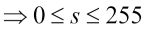
This means that a value of 0 in the input (black) gets mapped to 255 (white) and vice versa. Similarly, lighter shades of gray will yield the corresponding darker shades from the other end of the grayscale spectrum. If the range of the input values lie between 0 and 255, then the output will also lie within the same range. If you aren't convinced, here is some mathematical proof for you:

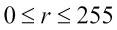(Assuming the input pixels are from an 8-bit grayscale color space)

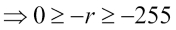(Multiplying by-1)

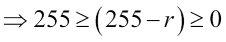(Adding 255)

Some books prefer to express the negative transformation as follows:

s=T(r)=(N-1-r)

Here, N is the number of grayscale levels in the color space we are dealing with. We have decided to stick with the former definition because all the color spaces we'll be dealing with in this book will involve values between 0 and 255. Hence, we can avoid the unnecessary fastidiousness.

The implementation of a lookup table for the negative transform is also fairly straightforward. We just replace the i with (255-i):

vector<uchar> getNegativeLUT() { 
  vector<uchar> LUT(256, 0); 
  for (int i = 0; i < 256; ++i) 
    LUT[i] = (uchar)(255 - i); 
  return LUT; 
} 

Let's run the code for negative transformation on some images and check what kind of an effect it produces:

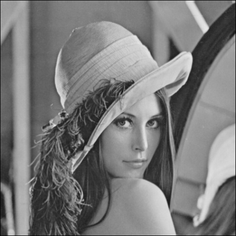
The preceding image serves as our input image and the output (negative transformed image) is as follows:.

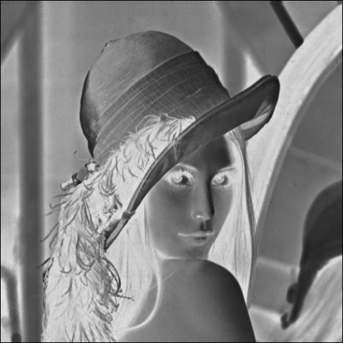
You can notice the darker pixels that make up the woman's hair (and feathers on the cap) have been transformed to white, and so have the eyes. The shoulders, which were on the fairer side of the spectrum, have been turned darker by the transform. You can now start to appreciate the kind of visual changes that this conceptually simple transformation seems to bring about in images! We iterate, once again, that the image manipulation apps, at the most basic, operate on similar principles.

If you are wondering who the lady in the image is, she goes by the name, Lena. Rather surprisingly, Lena's photograph with her iconic pose has become the de facto standard in the image processing community. A lot of literature in the field of image processing and computer vision uses this photo as an example to demonstrate the workings of some algorithm or technique. So, this is not the first time you'll be seeing her in this book!

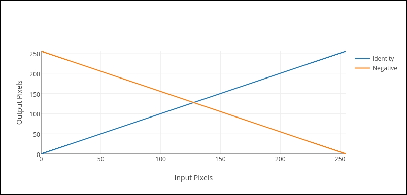
Before we finish the section on linear transformations, there is one more thought that I would like to leave you with. You might find some texts out there that like to visualize these transformations graphically as a plot between the input and output pixels. The reason that such visualization is made is because not all linear transformations are as simple as the ones discussed here. We will briefly discuss piecewise linear transformations, where a graphical plot provides a convenient medium to analyze the transformation. But, before that, you will find such a plot for both the identity and the negative transformation drawn on the same graph:

Both the linear transformations that we have discussed so far--identity and negative--are fairly trivial ones. You can have much more complicated forms for s=T(r). For example, instead of the transformation function being linear throughout the entire domain (0 to 255), we can make it piecewise linear. That would mean splitting the input domain into multiple, contiguous ranges and defining a linear transformation for each range, something along the lines of this:

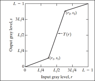
If you are wondering what purpose such a transformation achieves, the answer to that is contrast enhancement. When we say that an image has poor contrast, we mean that some (or all) parts of the image are not clearly distinguishable from their surroundings and neighbors. This happens when the pixels that make up the part of the image all belong to a very narrow band of intensity values. In the graph, consider the portion of the input intensity values that lie around L/2. You will notice that the narrow range of input pixels are mapped to a much wider range of output intensity values. This has been made possible by the steep line (greater slope), which defines the linear transformation around that region. As a result, all pixels that have intensity values within that range will get mapped to the wider output range, thereby improving the contrast of the image.

Now, astute readers might have realized that the shape of the piecewise linear transformation is dependent on the position of the points  and  So, how do we decide the location of the two points? Unfortunately, there is no single, specific answer to this question. As you will learn throughout the course of this book, in most cases, there can be no global correct answer for the selection of such parameters in image processing or computer vision. It depends on the kind of data (within the domain of computer vision, data often equates to images) that we are given to work with.

It would be a good exercise to try and implement the lookup table for a piecewise linear transformation. You can control the shape of the curve by varying the position of the two points and try to see what kind of an effect it has on the algorithm performance.