Design and develop advanced computer vision projects using OpenCV with Python About This Book Program advanced computer vision applications in Python using different features of the OpenCV library Practical end-to-end project covering an important computer vision problem All projects in the book include a step-by-step guide to create computer vision applications Who This Book Is For This book is for intermediate users of OpenCV who aim to master their skills by developing advanced practical applications. Readers are expected to be familiar with OpenCV’s concepts and Python libraries. Basic knowledge of Python programming is expected and assumed. 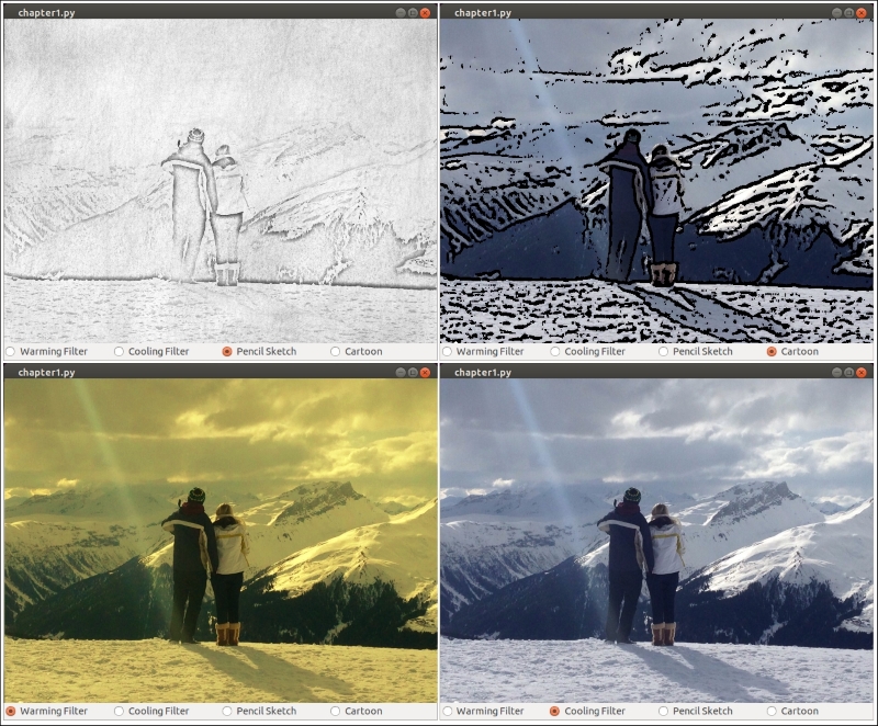What You Will Learn Generate real-time visual effects using different filters and image manipulation techniques such as dodging and burning Recognize hand gestures in real time and perform hand-shape analysis based on the output of a Microsoft Kinect sensor Learn feature extraction and feature matching for tracking arbitrary objects of interest Reconstruct a 3D real-world scene from 2D camera motion and common camera reprojection techniques Track visually salient objects by searching for and focusing on important regions of an image Detect faces using a cascade classifier and recognize emotional expressions in human faces using multi-layer peceptrons (MLPs) Recognize street signs using a multi-class adaptation of support vector machines (SVMs) Strengthen your OpenCV2 skills and learn how to use new OpenCV3 features In Detail OpenCV is a native cross platform C++ Library for computer vision, machine learning, and image processing. It is increasingly being adopted in Python for development. OpenCV has C++/C, Python, and Java interfaces with support for Windows, Linux, Mac, iOS, and Android. Developers using OpenCV build applications to process visual data; this can include live streaming data from a device like a camera, such as photographs or videos. OpenCV offers extensive libraries with over 500 functions This book demonstrates how to develop a series of intermediate to advanced projects using OpenCV and Python, rather than teaching the core concepts of OpenCV in theoretical lessons. Instead, the working projects developed in this book teach the reader how to apply their theoretical knowledge to topics such as image manipulation, augmented reality, object tracking, 3D scene reconstruction, statistical learning, and object categorization. By the end of this book, readers will be OpenCV experts whose newly gained experience allows them to develop their own advanced computer vision applications. Style and approach This book covers independent hands-on projects that teach important computer vision concepts like image processing and machine learning for OpenCV with multiple examples.