Linear algorithms are the ones where the work done varies in direct proportion with the input size, that is, if you double the input size, you double the work done. These typically involve a single pass through the input.

The problem presented in this example is that of counting the number of occurrences of a particular character in a string. Imagine we are given the string

, and we want to find out the number of occurrences of the letter a.

The following code in Snippet 1.5 goes through each character in the input string and if the character at the current position matches the search letter, a counter is increased. At the end of the loop, the final count is returned. The code is as follows:

public int countChars(char c, String str) {
  int count = 0;
  for (int i = 0; i < str.length(); i++) {
    if (str.charAt(i) == c) count++;
  }
  return count;
}

Snippet 1.5: Count the number of characters in a string. Source class name: CountChars.

Linear complexity algorithms are the most common types of algorithms. These usually make a single pass on the input and thus scale proportionally with the input size. In this section, we have seen one such example.

Quadratic complexity algorithms are not very performant for large input sizes. The work done increases following a quadratic proportion as we increase our input size. We already saw an example of a O(n²) in our minimum distance solution in Snippet 1.2. There are many other examples, such as bubble and selection sorting. The problem presented in this example is about finding the common elements contained in two arrays (assuming no duplicate values exist in each array), producing the intersection of the two inputs. This results in a runtime complexity of O(mn), where m and n are the sizes of the first and second input arrays. If the input arrays are the same size as n elements, this results in a runtime of O(n²). This can be demonstrated with the help of the following code:

public List<Integer> intersection(int[] a, int[] b) {
  List<Integer> result = new ArrayList<>(a.length);
  for (int x : a) {
    for (int y : b) {
      if (x == y) result.add(x);
    }
  }
  return result;
}

Snippet 1.6: Intersection between two arrays. Source class name:SimpleIntersection.

The amount of memory we use is dictated by the size of our result listed in our method. The bigger this list, the more memory we're using.

The best case is when we use the least amount of memory. This is when the list is empty, that is, when we have no common elements between the two arrays. Thus, this method has a best case space complexity of O(1), when there is no intersection.

The worst case is just the opposite, when we have all the elements in both arrays. This can happen when the arrays are equal to each other, although the numbers may be in a different order. The memory in this case is equal to the size of one of our input arrays. In short, the worst space complexity of the method is O(n).

In this section, we have shown examples of quadratic algorithms. Many other examples exist. In the next chapter, we will also describe a poorly-performing sorting algorithm, which is O(n²), called bubble sort.

Logarithmic complexity algorithms are very fast, and their performance hardly degrades as you increase the problem size. These types of algorithm scale really well. Code that has a runtime complexity of O(log n) is usually recognizable since it systematically divides the input in several steps. Common examples that operate in logarithmic times are database indexes and binary trees. If we want to find an item in a list, we can do it much more efficiently if the input list is sorted in some specific order. We can then use this ordering by jumping to specific positions of our list and skipping over a number of elements.

Snippet 1.7 shows an implementation of the binary search in Java. The method uses three array pointers—a start, an end, and a midpoint. The algorithm starts by checking the middle element in the array. If the element is not found and is less than the value at the middle, we choose to search in the lower half; otherwise, we choose the upper half. Figure 1.3 shows the steps involved when doing a binary search. The code snippet is as follows:

public boolean binarySearch(int x, int[] sortedNumbers) {
  int end = sortedNumbers.length - 1;
  int start = 0;
  while (start <= end) {
    int mid = (end - start) / 2 + start;
    if (sortedNumbers[mid] == x) return true;
    else if (sortedNumbers[mid] > x) end = mid - 1;
    else start = mid + 1;
  }
  return false;
}

Snippet 1.7: Binary search. Source class name:BinarySearch.

Take a look at the following diagram:

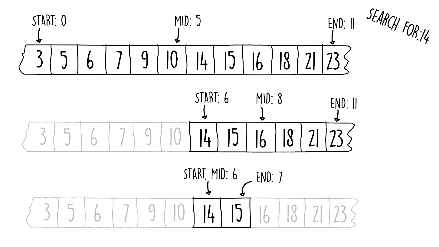
Figure 1.3: Binary search steps

Assuming the worst case scenario, how big would the input size have to be if our binary search algorithm is 95 array jumps (such as the one shown in Figure 1.3)? Since this is a binary search, where we're splitting the search space in two, we should use a logarithm of base 2.

Also, the inverse of a logarithm is the exponential. Thus, we can say the following:

Logarithmic algorithms are the opposite of exponential ones. As the input gets bigger, the rate of performance degradation gets smaller. This is a very desirable property as it means that our problem can scale to a huge size and would hardly affect our performance. In this section, we gave one such example of this class of complexity.

As we have seen previously, algorithms that have an exponential runtime complexity scale really poorly. There are many examples of problems for which only an O(kⁿ) solution is known. Improving these algorithms is a very dynamic area of study in computer science. Examples of these include the traveling salesman problem and cracking a password using a brute force approach. Now, let's see an example of such problem.

A prime number is only divisible by itself and one. The example problem we present here is called the prime factorization problem. It turns out that if you have the right set of prime numbers, you can create any other possible number by multiplying them all together. The problem is to find out these prime numbers. More specifically, given an integer input, find all the prime numbers that are factors of the input (primes that when multiplied together give us the input).

Snippet 1.8 shows one implementation for this problem, called trail division. If we take an input decimal number of n digits, this algorithm would perform in O(10ⁿ) in the worst case. The algorithm works by using a counter (called factor in Snippet 1.8) starting at two and checks whether if it's a factor of the input. This check is done by using the modulus operator. If the modulus operation leaves no remainder, then the value of the counter is a factor and is added to the factor list. The input is then divided by this factor. If the counter is not a factor (the mod operation leaves a remainder), then the counter is incremented by one. This continues until x is reduced to one. This is demonstrated by the following code snippet:

public List<Long> primeFactors(long x) {
  ArrayList<Long> result = new ArrayList<>();
  long factor = 2;
  while (x > 1) {
    if (x % factor == 0) {
      result.add(factor);
      x /= factor;
    } else {
      factor += 1;
    }
  }
  return result;
}

Snippet 1.8: Prime factors. Source class name:FindPrimeFactors.

Try executing the preceding code for the following two numbers:

Why does it take so long when you try the second number? What type of input triggers the worst-case runtime of this code?

The worst case of the algorithm is when the input is a prime number, wherein it needs to sequentially count all the way up to the prime number. This is what happens in the second input.

On the other hand, the largest prime factor for the first input is only 10,973, so the algorithm only needs to count up to this, which it can do quickly.

Exponential complexity algorithms are usually best avoided, and an alternate solution should be investigated. This is due to its really bad scaling with the input size. This is not to say that these types of algorithms are useless. They may be suitable if the input size is small enough or if it's guaranteed not to hit the worst case.

The efficiency of constant runtime algorithms remains fixed as we increase the input size. Many examples of these exist. Consider, for example, accessing an element in an array. Access performance doesn't depend on the size of the array, so as we increase the size of the array, the access speed stays constant.

Consider the code in Snippet 1.9. The number of operations performed remains constant, irrespective of the size of the input radius. Such an algorithm is said to have a runtime complexity of O(1). The code snippet is as follows:

private double circleCircumference(int radius) {
  return 2.0 * Math.PI * radius;
}

Snippet 1.9: Circle circumference. Source class name:CircleOperations.

Constant complexity algorithms are the most desirable out of all the complexity classes for the best scaling. Many of the simple mathematical functions, such as finding the distance between two points and mapping a three-dimensional coordinate to a two-dimensional one, all fall under this class.

public List<Integer> intersection(int[] a, int[] b)

public List<Integer> intersectionFast(int[] a, int[] b)

gradlew test --tests com.packt.datastructuresandalg.lesson1.activity.improveintersection*

public void mergeSort(int[] input) {
  Arrays.sort(input);
}