

Now that we have an understanding of today's hardware capabilities (multiple processors, multiple physical cores, and multiple logical cores (hardware threads)) and OS schedulers, let's discuss how to take advantage of this in our software development.
We know that our hardware has the ability to execute multiple instructions at the same time. As we will see in later chapters, .NET provides several classes and libraries that allow us to develop software that runs in multiple threads instead of a single software thread. The question is then, when does it make sense to develop our software to run in multiple threads concurrently and what kind of performance gains can we expect?
When designing for concurrency, we should look at a high-level abstraction of the application's requirements. Look at what functions the application performs and which functions can operate in parallel without affecting other functions. This will help us decide how to determine the amount of parallel operations we can design into the application. We will discuss in detail the .NET classes to implement both heavyweight concurrency (the Thread class) and lightweight concurrency (Task Parallel Library) in later chapters; but for now, we need to determine what and how much of our application can happen in parallel.
For example, if the application takes a list of items and encodes each item into an encrypted string, can the encoding of each item be run in parallel independent of the encoding of another item? If so, this "function" of the application is a good candidate for concurrency. Once you have defined all of the high-level functions an application must perform, this analysis will determine the amount of parallelism that the application can benefit from.
The following is a simple example of a parallel design where some of the functions operate sequentially and others in parallel. As we will see in the next section, once we can define how much of the application functions concurrently versus sequentially, then we can understand the performance gains we can expect.
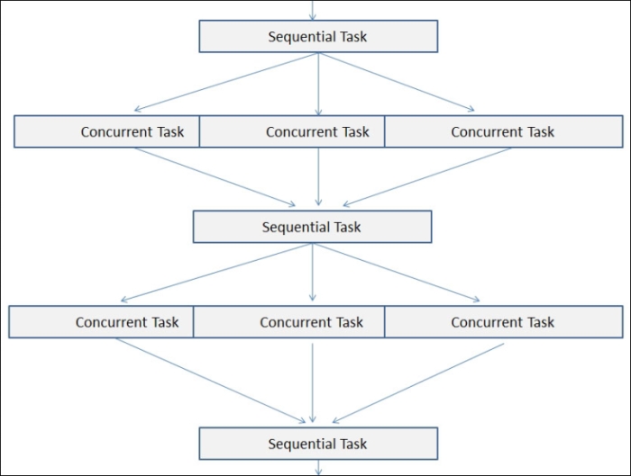
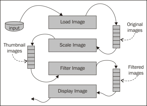
A lot of parallel designs employ some sort of pipelining design where some sequential work is performed, then some parallel work, then some sequential work, and so on. The preceding diagram shows a simple model for a pipeline design. Another popular concurrent design pattern is the producer-consumer model, which is really just a variation on the pipeline model. In this design, one function of the application produces an output that is consumed by another function of the application. The following is a diagram of this design pattern. In this example, each function can operate in parallel. The Load Image function produces image files to be consumed by the Scale Image function. The Scale Image function also produces thumbnail images to be consumed by the Filter Image function, and so on. Each of the function blocks can run in multiple concurrent threads because they are independent of each other:
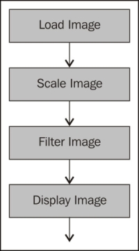
The following diagram illustrates the sequential operation:
The following diagram illustrates the parallel pipeline design:
One of the most common mistakes in designing or upgrading systems with multiple processors is making linear projections in their processing speed. It is very common to consider that each additional processor in the system will increase the performance in a way that is directly proportional to its processing capacity.
For instance, when we have a system with just one processor, and if we add three more, we will not have four times the performance. This is because each time we add a processor, the time they dedicate to coordinate their work and the task assignment process increases. Therefore, because of the increased processing power spent on managing tasks, their performance will not increase linearly.
The additional robots added to the kitchen must talk among themselves to coordinate their work.
The coordination costs and the performance increment depend upon a number of factors including the following:
The operating system and its management procedures to coordinate and distribute processes and threads among multiple processors: This is the robots' accuracy in assigning the appropriate task to the most capable robot model for that particular task.
The level of optimization to run multiple processors offered by applications: This is one of the most relevant points, even when we are using an n-way symmetric multiprocessing scheme. In this book, we will learn to reach high levels of optimizations for concurrency in our software. This can be correlated to the robots' abilities to work with other robots on the same tasks.
The microprocessors' microarchitecture: This corresponds to how fast the robots move their hands and legs, and do similar tasks.
The speed of the memory subsystem shared by the microprocessors: This is the robots' communications interface.
The speed of the I/O buses shared by the microprocessors: This is the robots' efficiency and precision in managing their hands and legs to do each task (mopping the floor and cooking, for example).
All these items represent a problem when we design or upgrade a machine, because we need answers to the following questions:
How many microprocessors do we need when the number of users increases? How many robots do you need according to the number of friends/tasks?
How many microprocessors do we need to increase an application's performance? How many robots do you need to accelerate the wash-up time?
How many microprocessors do we need to run a critical process within a specific time period? How many robots do you need to clean the oven in 5 minutes?
We need a reference, similar to the one offered in the following table, in which we can see the coordination cost and the relative performance for an increasing number of processors:
|
Number of processors |
Coordination cost |
Relative performance | ||
|---|---|---|---|---|
|
In relative processors |
In percentage |
In relative processors |
In percentage | |
|
1 |
0.00 |
0% |
1.00 |
100% |
|
2 |
0.09 |
5% |
1.91 |
95% |
|
3 |
0.29 |
10% |
2.71 |
90% |
|
4 |
0.54 |
14% |
3.46 |
86% |
|
5 |
0.84 |
17% |
4.16 |
83% |
|
6 |
1.17 |
19% |
4.83 |
81% |
|
7 |
1.52 |
22% |
5.48 |
78% |
|
8 |
1.90 |
24% |
6.10 |
76% |
|
9 |
2.29 |
25% |
6.71 |
75% |
|
10 |
2.70 |
27% |
7.30 |
73% |
|
11 |
3.12 |
28% |
7.88 |
72% |
|
12 |
3.56 |
30% |
8.44 |
70% |
|
13 |
4.01 |
31% |
8.99 |
69% |
|
14 |
4.47 |
32% |
9.53 |
68% |
|
15 |
4.94 |
33% |
10.06 |
67% |
|
16 |
5.42 |
34% |
10.58 |
66% |
|
17 |
5.91 |
35% |
11.09 |
65% |
|
18 |
6.40 |
36% |
11.60 |
64% |
|
19 |
6.91 |
36% |
12.09 |
64% |
|
20 |
7.42 |
37% |
12.58 |
63% |
|
21 |
7.93 |
38% |
13.07 |
62% |
|
22 |
8.46 |
38% |
13.54 |
62% |
|
23 |
8.99 |
39% |
14.01 |
61% |
|
24 |
9.52 |
40% |
14.48 |
60% |
|
25 |
10.07 |
40% |
14.93 |
60% |
|
26 |
10.61 |
41% |
15.39 |
59% |
|
27 |
11.16 |
41% |
15.84 |
59% |
|
28 |
11.72 |
42% |
16.28 |
58% |
|
29 |
12.28 |
42% |
16.72 |
58% |
|
30 |
12.85 |
43% |
17.15 |
57% |
|
31 |
13.42 |
43% |
17.58 |
57% |
|
32 |
14.00 |
44% |
18.00 |
56% |
This table was prepared taking into account an overall average performance test with many typical applications well optimized for multiprocessing, and the most modern processors with multiple execution cores used in workstations and servers. These processors were all compatible with AMD64 or EMT64 instruction sets, also known as x86-64. We can take these values as a reference in order to have an idea of the performance improvement that we will see in optimized applications.
As shown in the previous table, the coordination cost grows exponentially as the number of processors or cores increases. The following graph shows the relative performance versus the number of processors:
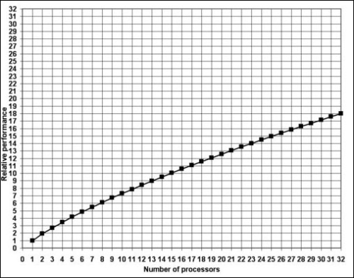
As we can see in the preceding screenshot, the relative performance grows logarithmically as the number of processors or cores increase.
Note
The following are the formulas used to calculate the values presented in the table and the graphs:
Coordination cost = 0.3 x logarithm (number of processors) x (number of processors - 1)
Relative performance = number of processors - coordination cost
The percentages are the result of the division between the coordination cost or the relative performance and the total number of microprocessors installed.
Nowadays, the problem is that without many concurrent users, multiple processor systems have not proved to be as useful as expected. The use of machines equipped with more than one processor in workstations used by just one user is meaningful only when the applications executed are designed to work with multiple processors.
Most applications designed for a single user are not optimized to take full advantage of multiple processors. Therefore, if the code is not prepared to use these additional processors, their performance will not improve, as was explained earlier.
But, why does this happen? The answer is simple. The process to develop applications that take full advantage of multiple processors is much more complex than traditional software development (this book will show how to make this task much easier). With the exception of specialized applications requiring a lot of processing capacity and those dedicated to resolving complex calculations, most applications have been developed using a traditional, linear programming scheme.
Nevertheless, the release of physical microprocessors with multiple logical execution cores lead to the widespread availability of multiprocessing systems and an urgent need to take full advantage of these microarchitectures.
A system with multiple processors can be analyzed and measured by the following items:
Total number of processors and their features: This is the total number of robots and their features.
Processing capacity (discounting the coordination overload): This is the robots' speed at working on each task (without communicating).
Microarchitecture and architecture: This is the number of execution cores in each physical microprocessor and the number of physical microprocessors with each microarchitecture. These are the subrobots in each robot, the number of hands, legs, and their speed.
Shared memory's bus bandwidth: This is the maximum number of concurrent communications that the robots can establish.
I/O bus bandwidth: This is the robots' efficiency, precision, and speed in managing their hands and legs concurrently to do each task.
Note
Bandwidth between processors
This bus allows the processors to establish a fluid communication between them. It is also known as the inter-processor bus. In some microarchitectures, this bus is the same as the FSB. It competes with the outputs to the microprocessors' outside world and therefore steals available bandwidth. The great diversity in microarchitectures makes it difficult to foretell the performance of the applications optimized for multiprocessing in every running context that is possible in the modern computing world.
We are considering neither the storage space nor the amount of memory. We are focused on the parameters that define the operation and the performance of multiple processors.
Amdahl's law is one of the two laws of parallel optimization that is used to help determine the expected performance gains with parallel computer designs, for both hardware and software.
Amdahl's law is a formula to help estimate the performance gains to be expected in an application given the amount of the application that is executed concurrently and the number of physical cores in the machine.
Gene Amdahl is a computer architect who in 1967 presented his algorithm to compute the maximum expected performance improvement that can be expected when part of a system is written for parallelism. The algorithm calculates the expected speedup as a percentage.
This law takes into account the number of physical cores of execution, N, the percentage, P, of the application that is concurrent, and the percentage, B, that is serial. The time it takes to process when N cores are being used is as follows:
T (N) = T(1) x (P + 1/Nx(1-N))
So, the maximum speedup (N) would be calculated as:
Speedup (N) = T(1)/T(N) = T(1)/T(1)(B+1/N(1-P)) = 1/(P+1/N(1-P))
So, Amdahl's law states that if, for example, 50 percent of an application is run sequentially, 50 percent is concurrent, and the computer has two cores, then the maximum speedup is:
Speedup = 1/((1-.50)+.5/2) = 1.333
So, if the task took 100 execution cycles sequentially, then it will take 75 cycles with 50 percent concurrency because 75 (work units) x 1.33333 (percentage speedup) = 100 (work units).
The following graph shows the predicted speed increase of an application based on the number of additional processors and the percentage of the code that can run in parallel:
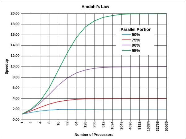
This law allows you to be able to estimate the performance gain of concurrency and to determine if the benefits are worth the extra complexity it adds to development, debug, and support. The extra costs of development, debug, and support have to be considered when developing a parallel software application.
Gustafson's law tries to address a shortfall of Amdahl's law by factoring in the scale of a problem. Gustafson was under the assumption that the problem size is not fixed but grows (scales). Amdahl's law calculates the speedup of a given problem size per the number of execution cores. Gustafson's law calculates a scaled speedup.
Gustafson's law is: S (P) = P – a * (P – 1) where S is the speedup percentage, P is the number of processing cores, and a is the percentage of concurrency of the application:
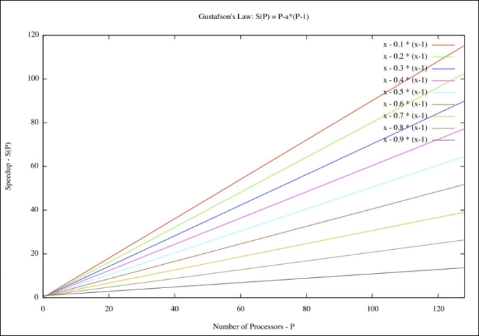
You will notice that the curves for a given percentage of concurrency do not level off in Gustafson's calculation versus Amdahl's.