

NumPy is the main foundation of the scientific Python ecosystem. This library offers a specific data structure for high-performance numerical computing: the multidimensional array. The rationale behind NumPy is the following: Python being a high-level dynamic language, it is easier to use but slower than a low-level language such as C. NumPy implements the multidimensional array structure in C and provides a convenient Python interface, thus bringing together high performance and ease of use. NumPy is used by many Python libraries. For example, pandas is built on top of NumPy.
In this recipe, we will illustrate the basic concepts of the multidimensional array. A more comprehensive coverage of the topic can be found in the Learning IPython for Interactive Computing and Data Visualization book.
Let's import the built-in
randomPython module and NumPy:In [1]: import random import numpy as npWe use the
%precisionmagic (defined in IPython) to show only three decimals in the Python output. This is just to reduce the number of digits in the output's text.In [2]: %precision 3 Out[2]: u'%.3f'
We generate two Python lists,
xandy, each one containing 1 million random numbers between 0 and 1:In [3]: n = 1000000 x = [random.random() for _ in range(n)] y = [random.random() for _ in range(n)] In [4]: x[:3], y[:3] Out[4]: ([0.996, 0.846, 0.202], [0.352, 0.435, 0.531])Let's compute the element-wise sum of all these numbers: the first element of
xplus the first element ofy, and so on. We use aforloop in a list comprehension:In [5]: z = [x[i] + y[i] for i in range(n)] z[:3] Out[5]: [1.349, 1.282, 0.733]How long does this computation take? IPython defines a handy
%timeitmagic command to quickly evaluate the time taken by a single statement:In [6]: %timeit [x[i] + y[i] for i in range(n)] 1 loops, best of 3: 273 ms per loop
Now, we will perform the same operation with NumPy. NumPy works on multidimensional arrays, so we need to convert our lists to arrays. The
np.array()function does just that:In [7]: xa = np.array(x) ya = np.array(y) In [8]: xa[:3] Out[8]: array([ 0.996, 0.846, 0.202])The
xaandyaarrays contain the exact same numbers that our original lists,xandy, contained. Those lists were instances of thelistbuilt-in class, while our arrays are instances of thendarrayNumPy class. These types are implemented very differently in Python and NumPy. In this example, we will see that using arrays instead of lists leads to drastic performance improvements.Now, to compute the element-wise sum of these arrays, we don't need to do a
forloop anymore. In NumPy, adding two arrays means adding the elements of the arrays component-by-component. This is the standard mathematical notation in linear algebra (operations on vectors and matrices):In [9]: za = xa + ya za[:3] Out[9]: array([ 1.349, 1.282, 0.733])We see that the
zlist and thezaarray contain the same elements (the sum of the numbers inxandy).Let's compare the performance of this NumPy operation with the native Python loop:
In [10]: %timeit xa + ya
100 loops, best of 3: 10.7 ms per loop
We observe that this operation is more than one order of magnitude faster in NumPy than in pure Python!
Now, we will compute something else: the sum of all elements in
xorxa. Although this is not an element-wise operation, NumPy is still highly efficient here. The pure Python version uses the built-insum()function on an iterable. The NumPy version uses thenp.sum()function on a NumPy array:In [11]: %timeit sum(x) # pure Python %timeit np.sum(xa) # NumPy 100 loops, best of 3: 17.1 ms per loop 1000 loops, best of 3: 2.01 ms per loopWe also observe an impressive speedup here also.
Finally, let's perform one last operation: computing the arithmetic distance between any pair of numbers in our two lists (we only consider the first 1000 elements to keep computing times reasonable). First, we implement this in pure Python with two nested
forloops:In [12]: d = [abs(x[i] - y[j]) for i in range(1000) for j in range(1000)] In [13]: d[:3] Out[13]: [0.230, 0.037, 0.549]Now, we use a NumPy implementation, bringing out two slightly more advanced notions. First, we consider a two-dimensional array (or matrix). This is how we deal with the two indices, i and j. Second, we use broadcasting to perform an operation between a 2D array and 1D array. We will give more details in the How it works... section.
In [14]: da = np.abs(xa[:1000,None] - ya[:1000])
In [15]: da
Out[15]: array([[ 0.23 ,  0.037,  ...,  0.542,  0.323,  0.473],
                 ...,
                [ 0.511,  0.319,  ...,  0.261,  0.042,  0.192]])
In [16]: %timeit [abs(x[i] - y[j])
                  for i in range(1000) for j in range(1000)]
         %timeit np.abs(xa[:1000,None] - ya[:1000])
1 loops, best of 3: 292 ms per loop
100 loops, best of 3: 18.4 ms per loop
Here again, we observe significant speedups.
A NumPy array is a homogeneous block of data organized in a multidimensional finite grid. All elements of the array share the same data type, also called dtype (integer, floating-point number, and so on). The shape of the array is an n-tuple that gives the size of each axis.
A 1D array is a vector; its shape is just the number of components.
A 2D array is a matrix; its shape is (number of rows, number of columns).
The following figure illustrates the structure of a 3D (3, 4, 2) array that contains 24 elements:
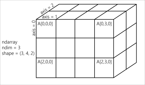
A NumPy array
The slicing syntax in Python nicely translates to array indexing in NumPy. Also, we can add an extra dimension to an existing array, using None or np.newaxis in the index. We used this trick in our previous example.
Element-wise arithmetic operations can be performed on NumPy arrays that have the same shape. However, broadcasting relaxes this condition by allowing operations on arrays with different shapes in certain conditions. Notably, when one array has fewer dimensions than the other, it can be virtually stretched to match the other array's dimension. This is how we computed the pairwise distance between any pair of elements in xa and ya.
How can array operations be so much faster than Python loops? There are several reasons, and we will review them in detail in Chapter 4, Profiling and Optimization. We can already say here that:
In NumPy, array operations are implemented internally with C loops rather than Python loops. Python is typically slower than C because of its interpreted and dynamically-typed nature.
The data in a NumPy array is stored in a contiguous block of memory in RAM. This property leads to more efficient use of CPU cycles and cache.
There's obviously much more to say about this subject. Our previous book, Learning IPython for Interactive Computing and Data Visualization, contains more details about basic array operations. We will use the array data structure routinely throughout this book. Notably, Chapter 4, Profiling and Optimization, covers advanced techniques of using NumPy arrays.
Here are some more references:
Introduction to the
ndarrayon NumPy's documentation available at http://docs.scipy.org/doc/numpy/reference/arrays.ndarray.htmlTutorial on the NumPy array available at http://wiki.scipy.org/Tentative_NumPy_Tutorial
The NumPy array in the SciPy lectures notes present at http://scipy-lectures.github.io/intro/numpy/array_object.html
The Getting started with exploratory data analysis in IPython recipe
The Understanding the internals of NumPy to avoid unnecessary array copying recipe in Chapter 4, Profiling and Optimization