Overfitting (one word) is such an important concept that I decided to start discussing it very early in the book.

If we go through many practice questions for an exam, we may start to find ways to answer questions which have nothing to do with the subject material. For instance, given only five practice questions, we find that if there are two potato and one tomato in a question, the answer is always A, if there are one potato and three tomato in a question, the answer is always B, then we conclude this is always true and apply such theory later on even though the subject or answer may not be relevant to potatoes or tomatoes. Or even worse, you may memorize the answers for each question verbatim. We can then score high on the practice questions; we do so with the hope that the questions in the actual exams will be the same as practice questions. However, in reality, we will score very low on the exam questions as it is rare that the exact same questions will occur in the actual exams.

The phenomenon of memorization can cause overfitting. We are over extracting too much information from the training sets and making our model just work well with them, which is called low bias in machine learning. However, at the same time, it will not help us generalize with data and derive patterns from them. The model as a result will perform poorly on datasets that were not seen before. We call this situation high variance in machine learning.

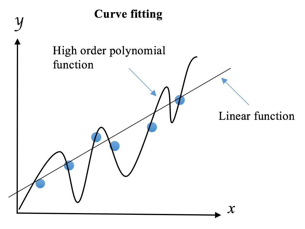
Overfitting occurs when we try to describe the learning rules based on a relatively small number of observations, instead of the underlying relationship, such the preceding potato and tomato example. Overfitting also takes place when we make the model excessively complex so that it fits every training sample, such as memorizing the answers for all questions as mentioned previously.

The opposite scenario is called underfitting. When a model is underfit, it does not perform well on the training sets, and will not so on the testing sets, which means it fails to capture the underlying trend of the data. Underfitting may occur if we are not using enough data to train the model, just like we will fail the exam if we did not review enough material; it may also happen if we are trying to fit a wrong model to the data, just like we will score low in any exercises or exams if we take the wrong approach and learn it the wrong way. We call any of these situations high bias in machine learning, although its variance is low as performance in training and test sets are pretty consistent, in a bad way.

We want to avoid both overfitting and underfitting. Recall bias is the error stemming from incorrect assumptions in the learning algorithm; high bias results in underfitting, and variance measures how sensitive the model prediction is to variations in the datasets. Hence, we need to avoid cases where any of bias or variance is getting high. So, does it mean we should always make both bias and variance as low as possible? The answer is yes, if we can. But in practice, there is an explicit trade-off between themselves, where decreasing one increases the other. This is the so-called bias–variance tradeoff. Does it sound abstract? Let’s take a look at the following example.

We were asked to build a model to predict the probability of a candidate being the next president based on the phone poll data. The poll was conducted by zip codes. We randomly choose samples from one zip code, and from these, we estimate that there's a 61% chance the candidate will win. However, it turns out he loses the election. Where did our model go wrong? The first thing we think of is the small size of samples from only one zip code. It is the source of high bias, also because people in a geographic area tend to share similar demographics. However, it results in a low variance of estimates. So, can we fix it simply by using samples from a large number zip codes? Yes, but don’t get happy so early. This might cause an increased variance of estimates at the same time. We need to find the optimal sample size, the best number of zip codes to achieve the lowest overall bias and variance.
Minimizing the total error of a model requires a careful balancing of bias and variance. Given a set of training samples x_1, x_2, …, x_n and their targets y_1, y_2, …, y_n, we want to find a regression function, ŷ(x), which estimates the true relation y(x) as correctly as possible. We measure the error of estimation, how good (or bad) the regression model is by mean squared error (MSE):

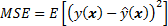
The E denotes the expectation. This error can be decomposed into bias and variance components following the analytical derivation as follows (although it requires a bit of basic probability theory to understand):

The bias term measures the error of estimations, and the variance term describes how much the estimation ŷ moves around its mean. The more complex the learning model ŷ(x) and the larger the size of training samples, the lower the bias will be. However, these will also create more shift on the model in order to fit better the increased data points. As a result, the variance will be lifted.
We usually employ the cross-validation technique to find the optimal model balancing bias and variance and to diminish overfitting.

The last term is the irreducible error.

Recall that between practice questions and actual exams, there are mock exams where we can assess how well we will perform in the actual ones and conduct necessary revision. In machine learning, the validation procedure helps evaluate how the models will generalize to independent or unseen datasets in a simulated setting. In a conventional validation setting, the original data is partitioned into three subsets, usually 60% for the training set, 20% for the validation set, and the rest 20% for the testing set. This setting suffices if we have enough training samples after partition and we only need a rough estimate of simulated performance. Otherwise, cross-validation is preferable.

In one round of cross-validation, the original data is divided into two subsets, for training and testing (or validation) respectively. The testing performance is recorded. Similarly, multiple rounds of cross-validation are performed under different partitions. Testing results from all rounds are finally averaged to generate a more accurate estimate of model prediction performance. Cross-validation helps reduce variability and therefore limit problems like overfitting.

There are mainly two cross-validation schemes in use, exhaustive and non-exhaustive. In the exhaustive scheme, we leave out a fixed number of observations in each round as testing (or validation) samples, the remaining observations as training samples. This process is repeated until all possible different subsets of samples are used for testing once. For instance, we can apply leave-one-out-cross-validation (LOOCV) and let each datum be in the testing set once. For a dataset of size n, LOOCV requires n rounds of cross-validation. This can be slow when n gets large.On the other hand, the non-exhaustive scheme, as the name implies, does not try out all possible partitions. The most widely used type of this scheme is k-fold cross-validation. The original data first randomly splits the data into k equal-sized folds. In each trail, one of these folds becomes the testing set, and the rest of the data becomes the training set. We repeat this process k times with each fold being the designated testing set once. Finally, we average the k sets of test results for the purpose of evaluation. Common values for k are 3, 5, and 10. The following table illustrates the setup for five folds:

We can also randomly split the data into training and testing set numerous times. This is formally called holdout method. The problem with this algorithm is that some samples may never end up in the testing set, while some may be selected multiple times in the testing set. Last but not least, nested cross-validation is a combination of cross-validations. It consists of the following two phases:

• The inner cross-validation, which is conducted to to find the best fit, and can be implemented as a k-fold cross-validation
• The outer cross-validation, which is used for performance evaluation and statistical analysis

We will apply cross-validation very intensively from Chapter 3, Spam Email Detection with Naive Bayes, to Chapter 7, Stock Price Prediction with Regression Algorithms. Before that, let’s see cross-validation through an analogy as follows, which will help us understand it better.

A data scientist plans to take his car to work, and his goal is to arrive before 9 am every day. He needs to decide the departure time and the route to take. He tries out different combinations of these two parameters on some Mondays, Tuesdays, and Wednesdays and records the arrival time for each trial. He then figures out the best schedule and applies it every day. However, it doesn’t work quite well as expected. It turns out the scheduling model is overfit with data points gathered in the first three days and may work well on Thursdays and Fridays. A better solution would be to test the best combination of parameters derived from Mondays to Wednesdays on Thursdays and Fridays and similarly repeat this process based on different sets of learning days and testing days of the week. This analogized cross-validation ensures the selected schedule work for the whole week.

In summary, cross-validation derives a more accurate assessment of model performance by combining measures of prediction performance on different subsets of data. This technique not only reduces variances and avoids overfitting but also gives an insight into how the model will generally perform in practice.

Another way of preventing overfitting is regularization. Recall that unnecessary complexity of the model is a source of overfitting just like cross-validation is a general technique to fight overfitting. Regularization adds extra parameters to the error function we are trying to minimize in order to penalize complex models.
According to the principle of Occam’s Razor, simpler methods are to be favored. William Occam was a monk and philosopher who, around 1320, came up with the idea that the simplest hypothesis that fits data should be preferred. One justification is that we can invent fewer simple models than complex models. For instance, intuitively, we know that there are more high-polynomial models than linear ones. The reason is that a line (y=ax+b) is governed by only two parameters--the intercept b and slope a. The possible coefficients for a line span a two-dimensional space. A quadratic polynomial adds an extra coefficient to the quadratic term, and we can span a three-dimensional space with the coefficients. Therefore, it is much easier to find a model that perfectly captures all the training data points with a high order polynomial function as its search space is much larger than that of a linear model. However, these easily-obtained models generalize worse than linear models, which are more prompt to overfitting. And of course, simpler models require less computation time. The following figure displays how we try to fit a linear function and a high order polynomial function respectively to the data:

The linear model is preferable as it may generalize better to more data points drawn from the underlying distribution. We can use regularization to reduce the influence of the high orders of polynomial by imposing penalties on them. This will discourage complexity, even though a less accurate and less strict rule is learned from the training data.

We will employ regularization quite often staring from Chapter 6, Click-Through Prediction with Logistic Regression. For now, let’s see the following analogy, which will help us understand it better:

A data scientist wants to equip his robotic guard dog the ability to identify strangers and his friends. He feeds it with the the following learning samples:

The robot may quickly learn the following rules: any middle-aged female of average height without glasses and dressed in black is a stranger; any senior short male without glasses and dressed in black is a stranger; anyone else is his friend. Although these perfectly fit the training data, they seem too complicated and unlikely to generalize well to new visitors. In contrast, the data scientist limits the learning aspects. A loose rule that can work well for hundreds of other visitors could be: anyone without glasses dressed in black is a stranger.

Besides penalizing complexity, we can also stop a training procedure early as a form of regularization. If we limit the time a model spends in learning or set some internal stopping criteria, it is more likely to produce a simpler model. The model complexity will be controlled in this way, and hence, overfitting becomes less probable. This approach is called early stopping in machine learning.

Last but not least, it is worth noting that regularization should be kept on a moderate level, or to be more precise, fine-tuned to an optimal level. Regularization, when too small, does has make any impact; regularization, when too large, will result in underfitting as it moves the model away from the ground truth. We will explore how to achieve the optimal regularization mainly in Chapter 6, Click-Through Prediction with Logistic Regression and Chapter 7, Stock Price Prediction with Regression Algorithms.