The following image shows a graph that represents a series of web pages (numbered from 1 to 8):

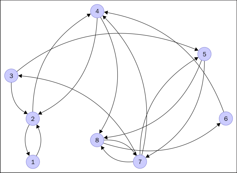
An arrow from a node to another indicates the existence of a link from the web page, represented by the sending node, to the page represented by the receiving node. For example, the arrow from node 2 to node 1 indicates that there is a link in web page 2 pointing to web page 1. Notice how web page 4 has two outer links (to pages 2 and 8), and there are three pages that link to web page 4 (pages 2, 6, and 7). The pages represented by nodes 2, 4, and 8 seem to be the most popular at first sight.

Is there a mathematical way to actually express the popularity of a web page within a network? Researchers at Google came up with the idea of a PageRank to roughly estimate this concept by counting the number and quality of links to a page. It goes like this:

Let us open an iPython session and load this particular matrix to memory.

In [1]: import numpy as np, matplotlib.pyplot as plt, \
   ...: scipy.linalg as spla, scipy.sparse as spsp, \
   ...: scipy.sparse.linalg as spspla
In [2]: np.set_printoptions(suppress=True, precision=3)
In [3]: cols = np.array([0,1,1,2,2,3,3,4,4,5,6,6,6,7,7]); \
   ...: rows = np.array([1,0,3,1,4,1,7,6,7,3,2,3,7,5,6]); \
   ...: data = np.array([1., 0.5, 0.5, 0.5, 0.5, \
   ...:                  0.5, 0.5, 0.5, 0.5, 1., \
   ...:                  1./3, 1./3, 1./3, 0.5, 0.5])
In [4]: T = np.zeros((8,8)); \
   ...: T[rows,cols] = data

From the transition matrix, we create a PageRank matrix G by fixing a positive constant p between 0 and 1, and following the formula G = (1-p)*T + p*B for a suitable damping factor p. Here, B is a matrix with the same size as T, with all its entries equal to 1/N. For example, if we choose p = 0.15, we obtain the following PageRank matrix:

In [5]: G = (1-0.15) * T + 0.15/8; \
   ...: print G
[[ 0.019  0.444  0.019  0.019  0.019  0.019  0.019  0.019]
 [ 0.869  0.019  0.444  0.444  0.019  0.019  0.019  0.019]
 [ 0.019  0.019  0.019  0.019  0.019  0.019  0.302  0.019]
 [ 0.019  0.444  0.019  0.019  0.019  0.869  0.302  0.019]
 [ 0.019  0.019  0.444  0.019  0.019  0.019  0.019  0.019]
 [ 0.019  0.019  0.019  0.019  0.019  0.019  0.019  0.444]
 [ 0.019  0.019  0.019  0.019  0.444  0.019  0.019  0.444]
 [ 0.019  0.019  0.019  0.444  0.444  0.019  0.302  0.019]]

PageRank matrices have some interesting properties:

A quick computation with scipy.linalg.eig finds that eigenvector for us:

In [6]: eigenvalues, eigenvectors = spla.eig(G); \
   ...: print eigenvalues
[ 1.000+0.j    -0.655+0.j    -0.333+0.313j -0.333-0.313j –0.171+0.372j -0.171-0.372j  0.544+0.j     0.268+0.j   ]
In [7]: PageRank = eigenvectors[:,0]; \
   ...: PageRank /= sum(PageRank); \
   ...: print PageRank.real
[ 0.117  0.232  0.048  0.219  0.039  0.086  0.102  0.157]

Those values correspond to the PageRank of each of the eight web pages depicted on the graph. As expected, the maximum value of those is associated to the second web page (0.232), closely followed by the fourth (0.219) and then the eighth web page (0.157). These values provide us with the information that we were seeking: the second web page is the most popular, followed by the fourth, and then, the eight.

The transition matrix is sparse: most of its entries are zeros. Sparse matrices with an extremely large size are of special importance in Numerical Linear Algebra, not only because they encode challenging scientific problems but also because it is extremely hard to manipulate them with basic algorithms.

Rather than storing to memory all values in the matrix, it makes sense to collect only the non-zero values instead, and use algorithms which exploit these smart storage schemes. The gain in memory management is obvious. These methods are usually faster for this kind of matrices and give less roundoff errors, since there are usually far less operations involved. This is another advantage of SciPy, since it contains numerous procedures to attack different problems where data is stored in this fashion. Let us observe its power with another example:

The University of Florida Sparse Matrix Collection is the largest database of matrices accessible online. As of January 2014, it contains 157 groups of matrices arising from all sorts of scientific disciplines. The sizes of the matrices range from very small (1 × 2) to insanely large (28 million × 28 million). More matrices are expected to be added constantly, as they arise in different engineering problems.

For example, the group with the most matrices in the database is the original Harwell-Boeing Collection, with 292 different sparse matrices. This group can also be accessed online at the Matrix Market: http://math.nist.gov/MatrixMarket/.

Each matrix in the database comes in three formats:

Let us import to our iPython session two matrices in the Matrix Market Exchange format from the collection, meant to be used in a solution of a least squares problem. These matrices are located at www.cise.ufl.edu/research/sparse/matrices/Bydder/mri2.html.The numerical values correspond to phantom data acquired on a Sonata 1.5-T scanner (Siemens, Erlangen, Germany) using a magnetic resonance imaging (MRI) device. The object measured is a simulation of a human head made with several metallic objects. We download the corresponding tar bundle and untar it to get two ASCII files:

The first twenty lines of the file mri2.mtx read as follows:

The first sixteen lines are comments, and give us some information about the generation of the matrix.

The seventeenth line indicates the size of the matrix, 63240 rows × 147456 columns, as well as the number of non-zero entries in the data, 569160.

The rest of the file includes precisely 569160 lines, each containing two integer numbers, and a floating point number: These are the locations of the non-zero elements in the matrix, together with the corresponding values.

A good way to read this file into ndarray is by means of the function loadtxt in NumPy. We can then use scipy to transform the array into a sparse matrix with the function coo_matrix in the module scipy.sparse (coo stands for the coordinate internal format).

In [8]: rows, cols, data = np.loadtxt("mri2.mtx", skiprows=17, \
   ...:                               unpack=True)
In [9]: rows -= 1; cols -= 1;
In [10]: MRI2 = spsp.coo_matrix((data, (rows, cols)), \
   ....:                        shape=(63240,147456))

The best way to visualize the sparsity of this matrix is by means of the routine spy from the module matplotlib.pyplot.

In [11]: plt.spy(MRI2); \
   ....: plt.show()

We obtain the following image. Each pixel corresponds to an entry in the matrix; white indicates a zero value, and non-zero values are presented in different shades of blue, according to their magnitude (the higher, the darker):

These are the first ten lines from the second file, mri2_b.mtx, which does not represent a sparse matrix, but a column vector:

%% MatrixMarket matrix array complex general
%-------------------------------------------------------------
% UF Sparse Matrix Collection, Tim Davis
% http://www.cise.ufl.edu/research/sparse/matrices/Bydder/mri2
% name: Bydder/mri2 : b matrix
%-------------------------------------------------------------
63240 1
-.07214859127998352 .037707749754190445
-.0729086771607399  .03763720765709877
-.07373382151126862 .03766685724258423

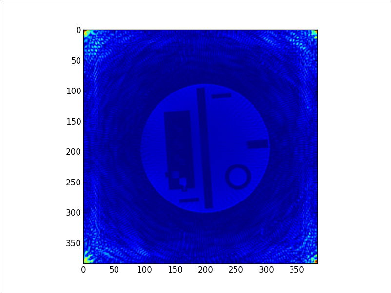
Those are six commented lines with information, one more line indicating the shape of the vector (63240 rows and 1 column), and the rest of the lines contain two columns of floating point values, the real and imaginary parts of the corresponding data. We proceed to read this vector to memory, solve the least squares problem suggested, and obtain the following reconstruction that represents a slice of the simulated human head:

In [12]: r_vals, i_vals = np.loadtxt("mri2_b.mtx", skiprows=7,
   ....:                             unpack=True)
In [13]: %time solution = spspla.lsqr(MRI2, r_vals + 1j*i_vals)
CPU times: user 4min 42s, sys: 1min 48s, total: 6min 30s
Wall time: 6min 30s
In [14]: from scipy.fftpack import fft2, fftshift
In [15]: img = solution[0].reshape(384,384); \
   ....: img = np.abs(fftshift(fft2(img)))
In [16]: plt.imshow(img); \
   ....: plt.show()

For matrices with a good structure, which are going to be exclusively involved in matrix multiplications, it is often possible to store the objects in smart ways. Let's consider an example.

A horizontal earthquake oscillation affects each floor of a tall building, depending on the natural frequencies of the oscillation of the floors. If we make certain assumptions, a model to quantize the oscillations on buildings with N floors can be obtained as a second-order system of N differential equations by competition: Newton's second law of force is set equal to the sum of Hooke's law of force, and the external force due to the earthquake wave.

These are the assumptions we will need:

Set M, the mass matrix, to be a diagonal matrix containing the floor masses on its diagonal. Set K, the Hooke's matrix, to be a tri-diagonal matrix with the following structure, for each row j, all the entries are zero except for the following ones:

Set H to be a column vector containing the external force on each floor due to the earthquake, and X, the column vector containing the functions x[j].

We have then the system: M * X'' = K * X + H. The homogeneous part of this system is the product of the inverse of M with K, which we denote as A.

To solve the homogeneous linear second-order system, X'' = A * X, we define the variable Y to contain 2*N entries: all N functions x[j], followed by their derivatives x'[j]. Any solution of this second-order linear system has a corresponding solution on the first-order linear system Y' = C * Y, where C is a block matrix of size 2*N × 2*N. This matrix C is composed by a block of size N × N containing only zeros, followed horizontally by the identity (of size N × N), and below these two, the matrix A followed horizontally by another N × N block of zeros.

It is not necessary to store this matrix C into memory, or any of its factors or blocks. Instead, we will make use of its structure, and use a linear operator to represent it. Minimal data is then needed to generate this operator (only the values of the masses and the Hooke's coefficients), much less than any matrix representation of it.

Let us show a concrete example with six floors. We indicate first their masses and Hooke's constants, and then, proceed to construct a representation of A as a linear operator:

In [17]: m = np.array([56., 56., 56., 54., 54., 53.]); \
   ....: k = np.array([561., 562., 560., 541., 542., 530.])
In [18]: def Axv(v):
   ....:     global k, m
   ....:     w = v.copy()
   ....:     w[0] = (k[1]*v[1] - (k[0]+k[1])*v[0])/m[0]
   ....:     for j in range(1, len(v)-1):
   ....:         w[j] = k[j]*v[j-1] + k[j+1]*v[j+1] - \
   ....:                (k[j]+k[j+1])*v[j]
   ....:         w[j] /= m[j]
   ....:     w[-1] = k[-1]*(v[-2]-v[-1])/m[-1]
   ....:     return w
   ....:
In [19]: A = spspla.LinearOperator((6,6), matvec=Axv, matmat=Axv,
   ....:                           dtype=np.float64)

The construction of C is very simple now (much simpler than that of its matrix!):

In [20]: def Cxv(v):
   ....:     n = len(v)/2
   ....:     w = v.copy()
   ....:     w[:n] = v[n:]
   ....:     w[n:] = A * v[:n]
   ....:     return w
   ....:
In [21]: C = spspla.LinearOperator((12,12), matvec=Cxv, matmat=Cxv,
   ....:                           dtype=np.float64)

A solution of this homogeneous system comes in the form of an action of the exponential of C: Y(t) = expm(C*t)* Y(0), where expm() here denotes a matrix exponential function. In SciPy, this operation is performed with the routine expm_multiply in the module scipy.sparse.linalg.

For example, in our case, given the initial value containing the values x[1](0)=0, ..., x[N](0)=0, x'[1](0)=1, ..., x'[N](0)=1, if we require a solution Y(t) for values of t between 0 and 1 in steps of size 0.1, we could issue the following:

In [22]: initial_condition = np.zeros(12); \
   ....: initial_condition[6:] = 1
In [23]: Y = spspla.exp_multiply(C, np.zeros(12), start=0,
   ....:                         stop=1, num=10)

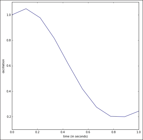
The oscillations of the six floors during the first second can then be calculated and plotted. For instance, to view the oscillation of the first floor, we could issue the following:

In [24]: plt.plot(np.linspace(0,1,10), Y[:,0]); \
   ....: plt.xlabel('time (in seconds)'); \
   ....: plt.ylabel('oscillation')

We obtain the following plot. Note how the first floor rises in the first tenth of a second, only to drop from 0.1 to 0.9 seconds from its original height to almost under a meter and then, start a slow rise:

These three examples illustrate the goal of this first chapter, Numerical Linear Algebra. In Python, this is accomplished first by storing the data in a matrix form, or as a related linear operator, by means of any of the following classes:

As we have seen in the examples, the choice of different classes obeys mainly to the sparsity of data and the algorithms that we are to apply to them.

This choice then dictates the modules that we use for the different algorithms: scipy.linalg for generic matrices and both scipy.sparse and scipy.sparse.linalg for sparse matrices or linear operators. These three SciPy modules are compiled on top of the highly optimized computer libraries BLAS (written in Fortran77), LAPACK (in Fortran90), ARPACK (in Fortran77), and SuperLU (in C).

Most of the routines in these three SciPy modules are wrappers to functions in the mentioned libraries. If we so desire, we also have the possibility to call the underlying functions directly. In the scipy.linalg module, we have the following:

For example, if we want to use the BLAS function NRM2 to compute Frobenius norms:

In [25]: blas_norm = spla.get_blas_func('nrm2')
In [26]: blas_norm(np.float32([1e20]))
Out[26]: 1.0000000200408773e+20