In this example, we need to generate a 100 random numbers and then plot the points in boxes.

Then, we mark the first outlier with it's identifier as follows:

> y <- rnorm(100)
> boxplot(y)
> identify(rep(1, length(y)), y, labels = seq_along(y))

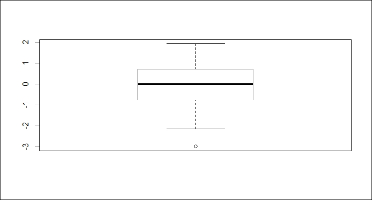
The boxplot function automatically computes the outliers for a set as well.

First, we will generate a 100 random numbers as follows (note that this data is randomly generated, so your results may not be the same):

> x <- rnorm(100)

We can have a look at the summary information on the set using the following code:

> summary(x)
    Min.  1st Qu.   Median     Mean  3rd Qu.     Max. 
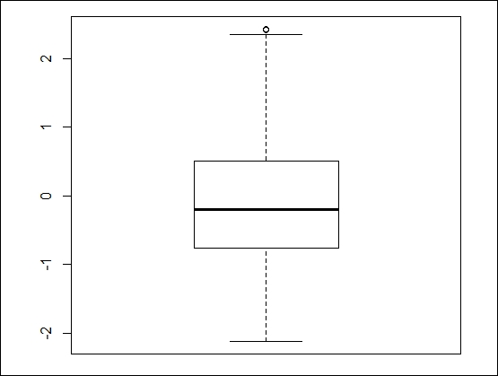
-2.12000 -0.74790 -0.20060 -0.01711  0.49930  2.43200

Now, we can display the outliers using the following code:

> boxplot.stats(x)$out
[1] 2.420850 2.432033

The following code will graph the set and highlight the outliers:

> boxplot(x)

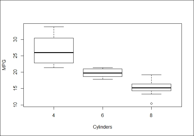
We can generate a box plot of more familiar data showing the same issue with outliers using the built-in data for cars, as follows:

boxplot(mpg~cyl,data=mtcars, xlab="Cylinders", ylab="MPG")

We can also use box plot's outlier detection when we have two dimensions. Note that we are forcing the issue by using a union of the outliers in x and y rather than an intersection. The point of the example is to display such points. The code is as follows:

> x <- rnorm(1000)
> y <- rnorm(1000)
> f <- data.frame(x,y)
> a <- boxplot.stats(x)$out
> b <- boxplot.stats(y)$out
> list <- union(a,b)
> plot(f)
> px <- f[f$x %in% a,]
> py <- f[f$y %in% b,]
> p <- rbind(px,py)
> par(new=TRUE)
> plot(p$x, p$y,cex=2,col=2)

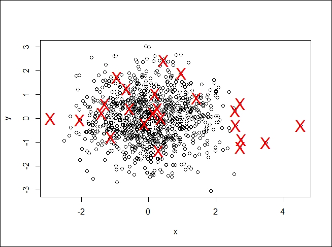
While R did what we asked, the plot does not look right. We completely fabricated the data; in a real use case, you would need to use your domain expertise to determine whether these outliers were correct or not.

We can use the name function to create our own anomaly as shown here:

name <- function(parameters,…) {
  # determine what constitutes an anomaly
  return(df)
}

Here, the parameters are the values we need to use in the function. I am assuming we return a data frame from the function. The function could do anything.

We will be using the iris data in this example, as shown here:

> data <- read.csv("http://archive.ics.uci.edu/ml/machine-learning-databases/iris/iris.data")

If we decide an anomaly is present when sepal is under 4.5 or over 7.5, we could use a function as shown here:

> outliers <- function(data, low, high) {
>  outs <- subset(data, data$X5.1 < low | data$X5.1 > high)
>  return(outs)
>}

Then, we will get the following output:

> outliers(data, 4.5, 7.5)
    X5.1 X3.5 X1.4 X0.2    Iris.setosa
8    4.4  2.9  1.4  0.2    Iris-setosa
13   4.3  3.0  1.1  0.1    Iris-setosa
38   4.4  3.0  1.3  0.2    Iris-setosa
42   4.4  3.2  1.3  0.2    Iris-setosa
105  7.6  3.0  6.6  2.1 Iris-virginica
117  7.7  3.8  6.7  2.2 Iris-virginica
118  7.7  2.6  6.9  2.3 Iris-virginica
122  7.7  2.8  6.7  2.0 Iris-virginica
131  7.9  3.8  6.4  2.0 Iris-virginica
135  7.7  3.0  6.1  2.3 Iris-virginica

This gives us the flexibility of making slight adjustments to our criteria by passing different parameter values to the function in order to achieve the desired results.

Another popular package is DMwR. It contains the lofactor function that can also be used to locate outliers. The DMwR package can be installed using the following command:

> install.packages("DMwR")
> library(DMwR)

We need to remove the species column from the data, as it is categorical against it data. This can be done by using the following command:

> nospecies <- data[,1:4]

Now, we determine the outliers in the frame:

> scores <- lofactor(nospecies, k=3)

Next, we take a look at their distribution:

> plot(density(scores))

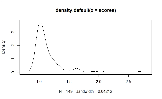
One point of interest is if there is some close equality amongst several of the outliers (that is, density of about 4).