If you remember, we saw that it is possible to represent really advanced concepts using a probability distribution; when we have many random variables, we call this distribution a joint distribution. Sometimes it is not impossible to have hundreds if not thousands or more of those random variables. Representing such a big distribution is extremely hard and in most cases impossible.

For example, in medical diagnoses, each random variable could represent a symptom. We can have dozens of them. Other random variables could represent the age of the patient, the gender of the patient, his or her temperature, blood pressure, and so on. We can use many different variables to represent the health state of a patient. We can also add other information such as recent weather conditions, the age of the patient, and his or her diet.

Then there are two tasks we want to solve with such a complex system:

However, there is something important: in such a model we would like to use another important piece of knowledge, maybe one of the most important: interactions between the various components—in other words, dependencies between the random variables. For example, there are obvious dependencies between symptoms and disease. On the other end, diet and symptoms can have a more distant dependency or can be dependent through another variable such as age or gender.

Finally, all the reasoning that is done with such a model is probabilistic in nature. From the observation of a variable X, we want to infer the posterior distribution of some other variables and have their probability rather than a simple yes or no answer. Having a probability gives us a richer answer than a binary response.

Let's make a simple computation. Imagine we have two binary random variables such as the one we saw in the previous section of this chapter. Let's call them X and Y. The joint probability distribution over these two variables is P(X,Y). They are binary so they can take two values each, which we will call x₁,x₂ and y₁,y₂, for the sake of clarity.

How many probability values do we need to specify? Four in total for P(X=x₁,Y=y₁), P(X=x₁,Y=y₂), P(X=x₂,Y=y₁), and P(X=x₂,Y=y₂).

Let's say we have now not two binary random variables, but ten. It's still a very simple model, isn't it? Let's call the variables X₁,X₂,X₃,X₄,X₅,X₆,X₇,X₈,X₉,X₁₀. In this case, we need to provide 2¹⁰ = 1024 values to determine our joint probability distribution. And what if we add another 10 variables for a total of 20 variables? It's still a very small model. But we need to specify 2²⁰ = 1048576 values. This is more than a million values. So for such a simple model, the task becomes simply impossible!

Probabilistic graphical models is the right framework to describe such models in a compact way and allow their construction and use in a most efficient manner. In fact, it is not unheard of to use probabilistic graphical models with thousands of variables. Of course, the computer model doesn't store billions of values, but in fact uses conditional independence in order to make the model tractable and representable in a computer's memory. Moreover, conditional independence adds structural knowledge to the model, which can make a massive difference.

In a probabilistic graphical model, such knowledge between variables can be represented with a graph. Here is an example from the medical world: how to diagnose a cold. This is just an example and by no means medical advice. It is over-simplified for the sake of simplicity. We have several random variables such as:

Because each of the symptoms can exist in different degrees, it is natural to represent the variables as random variables. For example, if the patient's nose is a bit blocked, we will assign a probability of, say, 60% to this variable, that is P(N=blocked)=0.6 and P(N=not blocked)=0.4.

In this example, the probability distribution P(Se,N,H,S,C,Cold) will require 4 * 2⁵ = 128 values in total (4 seasons and 2 values for each other random variables). It's quite a lot and honestly it's quite hard to determine things such as the probability that the nose is not blocked and that the patient has a headache and sneezes and so on.

However, we can say that a headache is not directly related to a cough or a blocked nose, except when the patient has a cold. Indeed, the patient could have a headache for many other reasons.

Moreover, we can say that the Season has quite a direct effect on Sneezing, Blocked Nose, or Cough but less or none on Headache. In a probabilistic graphical model, we will represent these dependency relationships with a graph, as follows, where each random variable is a node in the graph and each relationship is an arrow between two nodes:

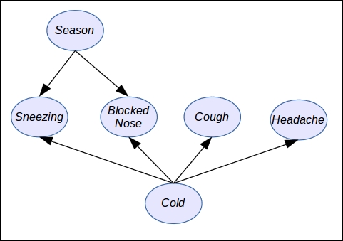
As you can see in the preceding figure, there is a direct relationship between each node and each variable of the probabilistic graphical model and also a direct relationship between arrows and the way we can simplify the joint probability distribution in order to make it tractable.

Using a graph as a model to simplify a complex (and sometimes complicated) distribution presents numerous benefits:

In the previous example on the diagnosis of the common cold, we defined a simple model with a few variables Se, N, H, S, C, and R. We saw that, for such a simple expert system, we needed 128 parameters!

We also saw that we can make a few independence assumptions based only on common sense or common knowledge. Later in this book, we will see how to discover those assumptions from a data set (also called structural learning).

So we can rewrite our joint probability distribution taking into account these assumptions as follows:

In this distribution, we did a factorization; that is, we expressed the original joint distribution as a product of factors. In this case, the factors are simpler probability distributions such as P(C | Cold), the probability of coughing given that one has a cold. And as we considered all the variables to be binary (except Season, which can take of course four values), each small factor (distribution) will need only a few parameters to be determined: 4 + 2³ + 2³ + 2 +2² + 2² =30. Only 30 easy parameters instead of 128! It's a massive improvement.

I said the parameters are easy, because they're easy to determine, either by hand or from data. For example, we don't know if the patient has a cold or not, so we can assign equal probability to the variable Cold, that is P(Cold = true)=P(Cold = false)=0.5.

Similarly, it's easy to determine P(C | Cold) because, if the patient has a cold (Cold=true), he or she will likely cough. If he or she has no cold, then chances will be low for the patient to cough, but not zero because the cause could be something else.

In general, a directed probabilistic graphical model factorizes a joint distribution over the random variables X₁, X₂…X_n as follows:

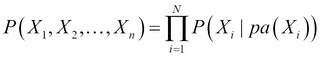
pa(X_i) is the subset of parent variables of the variable X_i as defined in the graph.

The parents are easy to read on a graph: when an arrow goes from A to B, then A is the parent of B. A node can have as many children as needed and a node can have as many parents as needed too.

Directed models are good for representing problems in which causality has to be modeled. It is also a good model for learning from parameters because each local probability distribution is easy to learn.

Several times in this chapter, we mentioned the fact that PGM can be built using simple blocks and assembled to make a bigger model. In the case of directed models, the blocks are the small probability distributions P(X_i | pa(X_i)).

Moreover, if one wants to extend the model by defining new variables and relations, it is as simple as extending the graph. The algorithms designed for directed PGM work for any graph, whatever its size.

Nevertheless, not all probability distributions can be represented by a directed PGM and sometimes it is necessary to relax certain assumptions.

Also it is important to note the graph must be acyclic. It means that you can't have an arrow from node A to node B and from node B to node A as in the following figure:

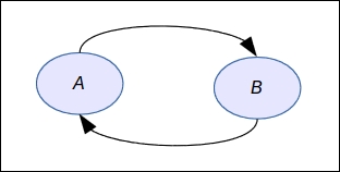
In fact, this graph does not represent a factorization at all as defined earlier and it would mean something like A is a cause of B while at the same time B is a cause of A. It's paradoxical and has no equivalent mathematical formula.

When the assumption or relationships are not directed, there exists a second form of probabilistic graphical model in which all the edges are undirected. It is called an undirected probabilistic graphical model or a Markov network.

An undirected probabilistic graphical model factorizes a joint distribution over the random variables X₁, X₂…X_n as follows:

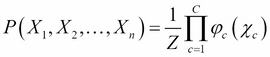
This formula needs a bit of explanation:

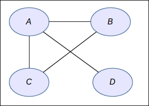
In the preceding figure, we have four nodes and the φ_c functions will be defined on the subsets that are maximal cliques—that is {ABC} and {A,D}. So the distribution is not very complex after all. This type of model is used a lot in applications such as computer vision, image processing, finance, and many more applications where the relationships between the variables follow a regular pattern.

It's about time to talk about the applications of probabilistic graphical models. There are so many applications that I would need another hundred pages to describe a subset of them. As we saw, it is a very powerful framework to model complex probabilistic models by making them easy to interpret and tractable.

In this section, we will use our two previous models: the light bulb machine and the cold diagnosis.

We recall that the cold diagnosis model has the following factorization:

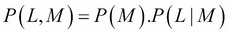
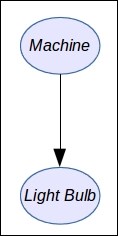
The light bulb machine, though, is defined by two variables only: L and M. And the factorization is very simple:

The graph corresponding to this distribution is simply:

In order to represent our probabilistic graphical model, we will use an R package called gRain. To install it:

source("http://bioconductor.org/biocLite.R")
biocLite()
install.packages("gRain")

Note that the installation can take several minutes because this package depends on many other packages (and especially one we will use often called gRbase) and provides the base functions for manipulating graphs.

When the package is installed, you can load the base package with:

library("gRbase")

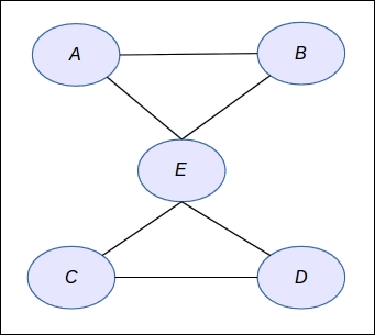
First of all, we want to define a simple undirected graph with five variables A, B, C, D and E:

graph <- ug("A:B:E + C:E:D")
class(graph)

We define a graph with a clique between A, B, and E, and another clique between C, E, and D. This will form a butterfly graph. The syntax is very simple: in the string each clique is separated by a + and each clique is defined by the name of each variable separated by a colon.

Next we need to install a graph visualization library. We will use the popular Rgraphviz and to install it you can enter:

install.packages("Rgraphviz")
plot(graph)

You will obtain your first undirected graph as follows:

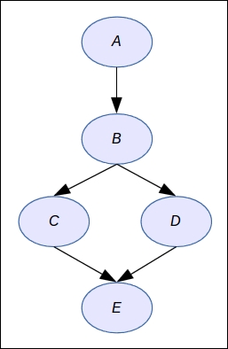
Next we want to define a directed graph. Let's say we have again the same {A,B,C,D,E} variables:

dag <- dag("A + B:A + C:B + D:B + E:C:D")
dag
plot(dag)

The syntax is again very simple: a node without parent comes alone such as A; otherwise parents are specified by the list of nodes separated by colons.

In this library, several syntaxes are available to define graphs, and you can also build them node by node. Throughout the book we will use several notations as well as a very important representation: the matrix notation. Indeed, a graph can be equivalently represented by a squared matrix where each row and each column represents a node and the coefficient in the matrix will be 1 is there is an edge; 0 otherwise. If the graph is undirected, the matrix will be symmetric; otherwise, the matrix can be anything.

Finally, with this second test we obtain the following graph:

Now we want to define a simple graph for the light bulb machine and provide numerical probabilities. Then we will do our computations again and check that the results are the same.

First we define the values for each node:

machine_val <- c("working","broken")
light_bulb_val <- c("good","bad")

Then we define the numerical values as percentages for the two random variables:

machine_prob <- c(99,1)
light_bulb_prob <- c(99,1,60,40)

The next step is to define the random variables with gRain:

M <- cptable(~machine, values=machine_prob, levels=machine_val)
L <- cptable(~light_bulb|machine, values=light_bulb_prob, levels=light_bulb_val)

Here, cptable means conditional probability table: it's a term to designate the memory representation of a probability distribution in the case of a discrete random variable. We will come back to this notion in Chapter 2, Exact Inference.

Finally, we can compile the new graphical model before using it. Again, this notion will make more sense in Chapter 2, Exact Inference. when we look at inference algorithms such as the Junction Tree Algorithm:

plist <- compileCPT(list(M,L))
plist

When printing the network, the result should be as follows:

CPTspec with probabilities:
 P( machine )
 P( light_bulb | machine )

Here, you clearly recognize the probability distributions that we defined earlier in this chapter.

If we print the variables' distribution we will find again what we had before:

plist$machine
plist$light_bulb

This will output the following result:

> plist$machine
machine
working  broken
   0.99    0.01
> plist$light_bulb
          machine
light_bulb working broken
      good    0.99    0.6
      bad     0.01    0.4

And now we ask the model the posterior probability. The first step is to enter an evidence into the model (that is to say that we observed a bad light bulb) by doing as follows:

net <- grain(plist)
net2 <- setEvidence(net, evidence=list(light_bulb="bad"))
querygrain(net2, nodes=c("machine"))

The library will compute the result by applying its inference algorithm and will output the following result:

$machine
machine
  working    broken
0.7122302 0.2877698

And this result is rigorously the same as we obtained with the Bayes method we defined earlier.

Therefore we are now ready to create more powerful models and explore the different algorithms suitable for solving different problems. This is what we're going to learn in the next chapter on exact inference in graphical models.