
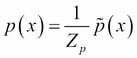
Suppose we want to sample from a distribution that is not a simple one. Let's call this distribution p(x) and let's assume we can evaluate p(x) for any given value x, up to a normalizing constant Z, that is:
In this context, p(x) is too complex to sample from but we have another simpler distribution q(x) from which we can draw samples. Next, we assume there exists a constant k such that 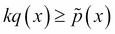 for all values of x. The function kq(x) is the comparison function as shown in the following figure:
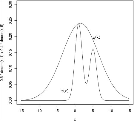
The distribution p(x) has been generated with a simple plot:
0.6*dnorm(x,1)+0.4*dnorm(x,5)
The rejection sampling algorithm is based on the following idea:
Draw a sample z0 from q(z), the proposal distribution
- Draw a second u0 sample from a uniform distribution on [0, kq(z0)]
-
If
 then the sample is rejected otherwise u0 is accepted
In the following figure, the pair (z0, u0) is rejected if it lies in the gray area. The accepted pairs are a uniform distribution under the curve of p(z) and therefore...