

IPython is an interactive shell with high-performance tools used for parallel and distributed computing. With the IPython Notebook, you can share code, text, mathematical expressions, plots, and other rich media with your target audience.
In this section, we will learn how to get started and run a simple IPython Notebook.
Depending on how you have installed Python on your machine, IPython might have been included in your Python environment. Please consult the IPython official documentation for the various installation methods most comfortable for you. The official page is available at http://ipython.org.
IPython can be downloaded from https://github.com/ipython. To install IPython, unpack the packages to a folder. From the terminal, navigate to the top-level source directory and run the following command:
$ python setup.py install
The
pip tool is a great way to install Python packages automatically. Think of it as a package manager for Python. For example, to install IPython without having to download all the source files, just run the following command in the terminal:
$ pip install ipython
To get pip to work in the terminal, it has to be installed as a Python module. Instructions for downloading and installing pip can be found at https://pypi.python.org/pypi/pip.
The IPython Notebook is the web-based interactive computing interface of IPython used for the whole computation process of developing, documenting, and executing the code. This section covers some of the common features in IPython Notebook that you may consider using for building financial applications.
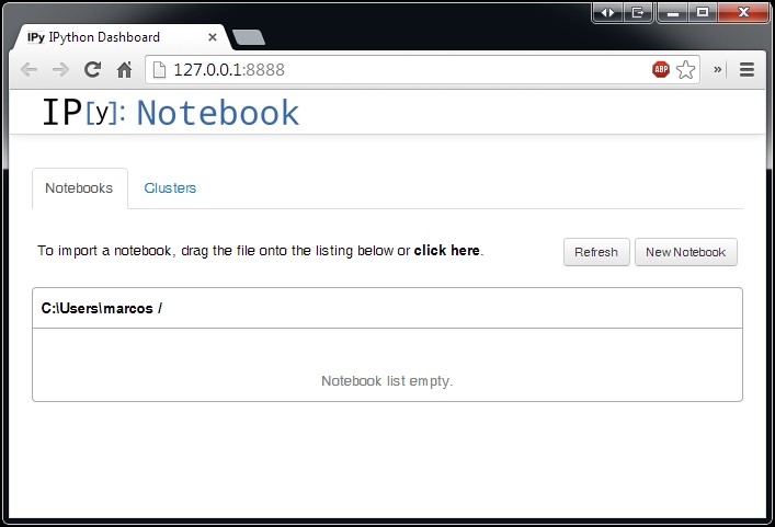
Here is a screenshot of the IPython Notebook in Windows OS:
Notebooks allow in-browser editing and executing of the code with the outputs attached to the code that generated them. It has the capability of displaying rich media, including images, videos, and HTML components.
Its in-browser editor allows the Markdown language that can provide rich text and commentary for the code.
Mathematical notations can be included with the use of LaTeX, rendered natively by MathJax. With the ability to import Python modules, publication-quality figures can be included inline and rendered using the matplotlib library.
Notebook documents are saved with the .ipynb extension. Each document contains everything related to an interactive session, stored internally in the JSON format. Since JSON files are represented in plain text, this allows notebooks to be version controlled and easily sharable.
Notebooks can be exported to a range of static formats, including HTML, LaTeX, PDF, and slideshows.
Notebooks can also be available as static web pages and served to the public via URLs using nbviewer (IPython Notebook Viewer) without users having to install Python. Conversion is handled using the nbconvert service.
Once you have IPython successfully installed in the terminal, type the following command:
$ ipython notebook
This will start the IPython Notebook server service, which runs in the terminal. By default, the service will automatically open your default web browser and navigate to the landing page. To access the notebook program manually, enter the http://localhost:8888 URL address in your web browser.
Tip
By default, a notebook runs in port 8888. To infer the correct notebook address, check the log output from the terminal.
The landing page of the notebook web application is called the dashboard, which shows all notebooks currently available in the notebook directory. By default, this directory is the one from which the notebook server was started.
Click on New Notebook from the dashboard to create a new notebook. You can navigate to the File | New menu option from within an active notebook:
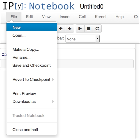
Here, you will be presented with the notebook name, a menu bar, a toolbar, and an empty code cell.
The menu bar presents different options that may be used to manipulate the way the notebook functions.
The toolbar provides shortcuts to frequently used notebook operations in the form of icons.
Each logical section in a notebook is known as a cell. A cell is a multi-line text input field that accepts plain text. A single notebook document contains at least one cell and can have multiple cells.
To execute the contents of a cell, from the menu bar, go to Cell | Run, or click on the Play button from the toolbar, or use the keyboard shortcut Shift + Enter.
Each cell can be formatted as a Code, Markdown, Raw NBConvert, or heading cell:
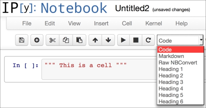
By default, each cell starts off as a code cell, which executes the Python code when you click on the Run button. Cells with a rounded rectangular box and gray background accept text inputs. The outputs of the executed box are displayed in the white space immediately below the text input.
Markdown cells accept the Markdown language that provides a simple way to format plain text into rich text. It allows arbitrary HTML code for formatting.
Mathematical notations can be displayed with standard LaTeX and AMS-LaTeX (the amsmath package). Surround the LaTeX equation with $ to display inline mathematics, and $$ to display equations in a separate block. When executed, MathJax will render Latex equations with high-quality typography.
Let's get started by creating a new notebook and populating it with some content. We will insert the various types of objects to demonstrate the various tasks.
We will begin by creating a new notebook by performing the following steps:
Click on New Notebook from the dashboard to create a new notebook. If from within an active notebook, navigate to the File | New menu option.
In the input field of the first cell, enter a page title for this notebook. In this example, type in
Welcome to Hello World.From the options toolbar menu, go to Cells | Cell Type and select Heading 1. This will format the text we have entered as the page title. The changes, however, will not be immediate at this time.
From the options toolbar menu, go to Insert | Insert Cell Below. This will create another input cell below our current cell.
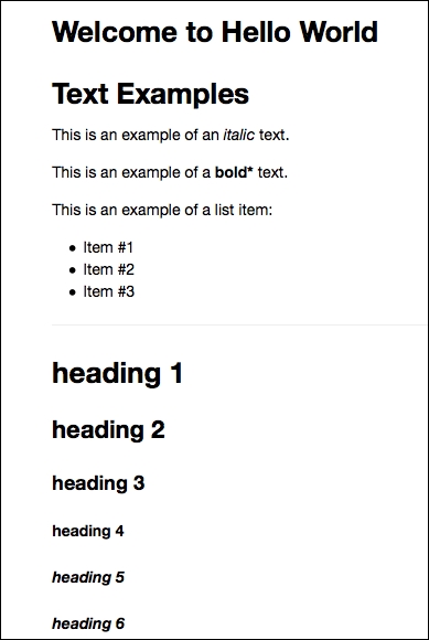
In this example, we will insert the following piece of text that contains the Markdown code:
Text Examples
===

This is an example of an *italic* text.

This is an example of a **bold*** text.

This is an example of a list item:
- Item #1
- Item #2
- Item #3

---

#heading 1
##heading 2
###heading 3
####heading 4
#####heading 5
######heading 6
From the toolbar, select Markdown instead of Code.
To run your code, go to Cell | Run All. This option will run all the Python commands and format your cells as required.
This will give us the following output:
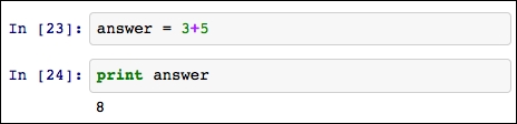
Let's perform a simple mathematical calculation in the notebook; let's add the numbers 3 and 5 and assign the result to the answer variable by typing in the code cell:
answer = 3 + 5
From the options menu, go to Insert | Insert Cell Below to add a new code cell at the bottom. We want to output the result by typing in the following code in the next cell:
print answer
Next, go to Cell | Run All. Our answer is printed right below the current cell.
The matplotlib module provides a MATLAB-like plotting framework in Python. With the matplotlib.pyplot function, charts can be plotted and rendered as graphic images for display in a web browser.
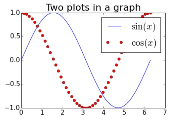
Let's demonstrate a simple plotting functionality of the IPython Notebook. In a new cell, paste the following code:
import numpy as np
import math
import matplotlib.pyplot as plt

x = np.linspace(0, 2*math.pi)
plt.plot(x, np.sin(x), label=r'$\sin(x)$')
plt.plot(x, np.cos(x), 'ro', label=r'$\cos(x)$')
plt.title(r'Two plots in a graph')
plt.legend()
The first three lines of the code contain the required import statements. Note that the NumPy, math, and matplotlib packages are required for the code to work in the IPython Notebook.
In the next statement, the variable x represents our x axis values from 0 through 7 in real numbers. The following statement plots the sine function for every value of x. The next plot command plots the cosine function for every value of x as a dotted line. The last two lines of the code print the title and legend respectively.
Running this cell gives us the following output:
What is TeX and LaTeX? TeX is the industry standard document markup language for math markup commands. LaTeX is a variant of TeX that separates the document structure from the content.
Mathematical equations can be displayed using LaTeX in the Markdown parser. The IPython Notebook uses MathJax to render LaTeX surrounded with $$ inside Markdown.
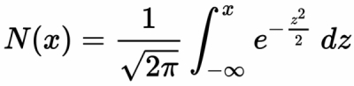
For this example, we will display a standard normal cumulative distribution function by typing in the following command in the cell:
$$N(x) = \frac{1}{\sqrt{2\pi}}\int_{-\infty}^{x} e^{- \frac{z^2}{2}}\, dz$$Select Markdown from the toolbar and run the current cell. This will transform the current cell into its respective equation output:
Besides using the MathJax typesetting, another way of displaying the same equation is using the math function of the IPython display module, as follows:
from IPython.display import Math
Math(r'N(x) = \frac{1}{\sqrt{2\pi}}\int_{-\infty}^{x} e^{- \frac{z^2}{2}}\, dz')
The preceding code will display the same equation, as shown in the following screenshot:

Notice that, since this cell is run as a normal code cell, the output equation is displayed immediately below the code cell.
We can also display equations inline with text. For example, we will use the following code with a single $ wrapping around the LaTeX expression:
This expression $\sqrt{3x-1}+(1+x)^2$ is an example of a TeX inline equationRun this cell as the Markdown cell. This will transform the current cell into the following:

To work with images, such as JPEG and PNG, use the Image class of the IPython display module. Run the following code to display a sample image:
from IPython.display import Image
Image(url='http://python.org/images/python-logo.gif')
On running the code cell, it will display the following output:
The
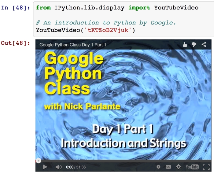
lib.display module of the IPython package contains a YouTubeVideo function, where you can embed videos hosted externally on YouTube into your notebook. For example, run the following code:
from IPython.lib.display import YouTubeVideo

# An introduction to Python by Google.
YouTubeVideo('tKTZoB2Vjuk')
The video will be displayed below the code, as shown in the following screenshot:
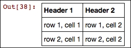
Notebook allows HTML representations to be displayed. One common use of HTML is the ability to display data with tables. The following code outputs a table with two columns and three rows, including a header row:
from IPython.display import HTML
table = """<table>
<tr>
<th>Header 1</th>
<th>Header 2</th>
</tr>
<tr>
<td>row 1, cell 1</td>
<td>row 1, cell 2</td>
</tr>
<tr>
<td>row 2, cell 1</td>
<td>row 2, cell 2</td>
</tr>
</table>"""
HTML(table)
The HTML function will render HTML tags as a string in its input argument. We can see the final output as follows:
In a notebook, pandas allow DataFrame objects to be represented as HTML tables.
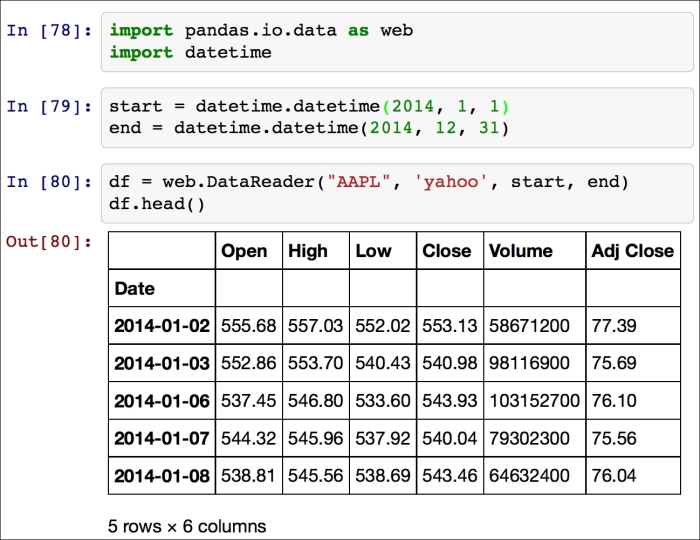
In this example, we will retrieve the stock market data from Yahoo! Finance and store them in a pandas DataFrame object with the help of the panas.io.data.web.DataReader function. Let's use the AAPL ticker symbol as the first argument, yahoo as its second argument, the start date of the market data as the third argument, and the end date as the last argument:
import pandas.io.data as web
import datetime

start = datetime.datetime(2014, 1, 1)
end = datetime.datetime(2014, 12, 31)
df = web.DataReader("AAPL", 'yahoo', start, end)
df.head()
With the df.head() command, the first five rows of the DataFrame object that contains the market data is displayed as an HTML table in the notebook:
You are now ready to place your code in a chronological order and present the key financial information, such as plots and data to your audience. Many industry practitioners use the IPython Notebook as their preferred editor for financial model development in helping them to visualize data better.
You are strongly encouraged to explore the powerful features the IPython Notebook has to offer that best suit your modeling needs. A gallery of interesting notebook projects used in scientific computing can be found at https://github.com/ipython/ipython/wiki/A-gallery-of-interesting-IPython-Notebooks.