Probability deals with the study of events. From our intuition, we can say that some events are more likely than others, but to quantify the likeliness of a particular event, we require the probability theory. It helps us predict the future by assessing how likely the outcomes are.

Before going deeper into the probability theory, let's first get acquainted with the basic terminologies and definitions of the probability theory. A random variable is a way of representing an attribute of the outcome. Formally, a random variable X is a function that maps a possible set of outcomes Ω to some set E, which is represented as follows:

X : Ω → E

As an example, let us consider the outing example again. To decide whether to go or not, we may consider the skycover (to check whether it is cloudy or not). Skycover is an attribute of the day. Mathematically, the random variable skycover (X) is interpreted as a function, which maps the day (Ω) to its skycover values (E). So when we say the event X = 40.1, it represents the set of all the days {ω} such that , where is the mapping function. Formally speaking, .

Random variables can either be discrete or continuous. A discrete random variable can only take a finite number of values. For example, the random variable representing the outcome of a coin toss can take only two values, heads or tails; and hence, it is discrete. Whereas, a continuous random variable can take infinite number of values. For example, a variable representing the speed of a car can take any number values.

For any event whose outcome is represented by some random variable (X), we can assign some value to each of the possible outcomes of X, which represents how probable it is. This is known as the probability distribution of the random variable and is denoted by P(X).

For example, consider a set of restaurants. Let X be a random variable representing the quality of food in a restaurant. It can take up a set of values, such as {good, bad, average}. P(X), represents the probability distribution of X, that is, if P(X = good) = 0.3, P(X = average) = 0.5, and P(X = bad) = 0.2. This means there is 30 percent chance of a restaurant serving good food, 50 percent chance of it serving average food, and 20 percent chance of it serving bad food.

In most of the situations, we are rather more interested in looking at multiple attributes at the same time. For example, to choose a restaurant, we won't only be looking just at the quality of food; we might also want to look at other attributes, such as the cost, location, size, and so on. We can have a probability distribution over a combination of these attributes as well. This type of distribution is known as joint probability distribution. Going back to our restaurant example, let the random variable for the quality of food be represented by Q, and the cost of food be represented by C. Q can have three categorical values, namely {good, average, bad}, and C can have the values {high, low}. So, the joint distribution for P(Q, C) would have probability values for all the combinations of states of Q and C. P(Q = good, C = high) will represent the probability of a pricey restaurant with good quality food, while P(Q = bad, C = low) will represent the probability of a restaurant that is less expensive with bad quality food.

Let us consider another random variable representing an attribute of a restaurant, its location L. The cost of food in a restaurant is not only affected by the quality of food but also the location (generally, a restaurant located in a very good location would be more costly as compared to a restaurant present in a not-very-good location). From our intuition, we can say that the probability of a costly restaurant located at a very good location in a city would be different (generally, more) than simply the probability of a costly restaurant, or the probability of a cheap restaurant located at a prime location of city is different (generally less) than simply probability of a cheap restaurant. Formally speaking, P(C = high | L = good) will be different from P(C = high) and P(C = low | L = good) will be different from P(C = low). This indicates that the random variables C and L are not independent of each other.

These attributes or random variables need not always be dependent on each other. For example, the quality of food doesn't depend upon the location of restaurant. So, P(Q = good | L = good) or P(Q = good | L = bad)would be the same as P(Q = good), that is, our estimate of the quality of food of the restaurant will not change even if we have knowledge of its location. Hence, these random variables are independent of each other.

In general, random variables can be considered as independent of each other, if:

They may also be considered independent if:

We can easily derive this conclusion. We know the following from the chain rule of probability:

P(X, Y) = P(X) P(Y | X)

If Y is independent of X, that is, if X | Y, then P(Y | X) = P(Y). Then:

P(X, Y) = P(X) P(Y)

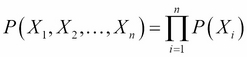
Extending this result on multiple variables, we can easily get to the conclusion that a set of random variables are independent of each other, if their joint probability distribution is equal to the product of probabilities of each individual random variable.

Sometimes, the variables might not be independent of each other. To make this clearer, let's add another random variable, that is, the number of people visiting the restaurant N. Let's assume that, from our experience we know the number of people visiting only depends on the cost of food at the restaurant and its location (generally, lesser number of people visit costly restaurants). Does the quality of food Q affect the number of people visiting the restaurant? To answer this question, let's look into the random variable affecting N, cost C, and location L. As C is directly affected by Q, we can conclude that Q affects N. However, let's consider a situation when we know that the restaurant is costly, that is, C = high and let's ask the same question, "does the quality of food affect the number of people coming to the restaurant?". The answer is no. The number of people coming only depends on the price and location, so if we know that the cost is high, then we can easily conclude that fewer people will visit, irrespective of the quality of food. Hence, .

This type of independence is called conditional independence.