
In the restaurant example or the late-for-school example, we used the Bayesian network to represent the independencies in the random variables. We also saw that we can use the Bayesian network to represent the joint probability distribution over all the variables using the chain rule. In this section, we will unify these two concepts and show that a probability distribution D can only be represented using a graph G, if and only if D can be represented as a set of CPDs associated with the graph G.
A graph object G is called an IMAP of a probability distribution D if the set of independency assertions in G, denoted by I(G), is a subset of the set of independencies in D, denoted by I(D).
Let's take an example of two random variables X and Y with the following two different probability distributions over it:
|
X |
Y |
P(X, Y) |
|---|---|---|
|
|
|
0.25 |
|
|
|
0.25 |
|
|
|
0.25 |
|
|
|
0.25 |


In this distribution, we can see that P(X) = 0.5 and P(Y) = 0.5. Also, P(X, Y) = P(X)P(Y). Hence, the two random variables X and Y are independent. If we try to represent any two random variables using a network, we have three possibilities:
A graph with two disconnected nodes X and Y
A graph with an edge from X → Y
A graph with an edge from Y → X
We can see from the previous distribution that 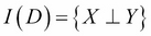 . In the case of disconnected nodes, we also have
 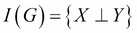 , whereas for the other two graphs, we have I(G) =
 . Hence, all the three graphs are IMAPS of the distribution, and any of these can be used to represent the probability distribution. However, the graph with both nodes disconnected is able to best represent the probability distribution and is known as the Perfect Map.
The structure of the Bayesian network encodes the independencies between the random variables, and every probability distribution for which this BN is an IMAP needs to satisfy these independencies. This allows us to represent the joint probability distribution in a very compact form.
Taking the example of the late-for-school model, using the chain rule, we can show that for any distribution, the joint probability distribution would be as follows:
P(A, R, J, L, S, Q) = P(A) × P(R|A) × P(J|A, R) × P(L|A, R, J) × P(S|A, R, J, L) ×
P(Q|A, R, J, L, S)
However, if we consider a distribution for which the BN is an IMAP, we get information about the independencies in the distribution. As we can see in this example, we know from the Bayesian network structure that S is independent of A and R, given J and L; Q is independent of A, R, and L, and S, given J; and so on. Applying all these conditions on the equation for joint probability distribution reduces it to the following:
P(A, R, J, L, S, Q) = P(A) × P(R) × P(J|A, R) × P(L) × P(S|J, L) × P(Q|J)
Every graph object has associated independencies with it. These independencies allow us to represent the joint probability distribution of the BN in a compact form.