

A histogram will tell you approximately how data is distributed throughout its range, and provide a visual means of classifying your data into one of a handful of common distributions. Many distributions occur frequently in data analysis, but none so much as the normal distribution, also called the Gaussian distribution.
Note
The distribution is named the normal distribution because of how often it occurs in nature. Galileo noticed that the errors in his astronomical measurements followed a distribution where small deviations from the mean occurred more frequently than large deviations. It was the great mathematician Gauss' contribution to describing the mathematical shape of these errors that led to the distribution also being called the Gaussian distribution in his honor.
A distribution is like a compression algorithm: it allows a potentially large amount of data to be summarized very efficiently. The normal distribution requires just two parameters from which the rest of the data can be approximated—the mean and the standard deviation.
The reason for the normal distribution's ubiquity is partly explained by the central limit theorem. Values generated from diverse distributions will tend to converge to the normal distribution under certain circumstances, as we will show next.
A common distribution in programming is the uniform distribution. This is the distribution of numbers generated by Clojure's rand function: for a fair random number generator, all numbers have an equal chance of being generated. We can visualize this on a histogram by generating a random number between zero and one many times over and plotting the results.
(defn ex-1-15 []
  (let [xs (->> (repeatedly rand)
                (take 10000))]
    (-> (c/histogram xs
                     :x-label "Uniform distribution"
                     :nbins 20)
        (i/view))))
The preceding code will generate the following histogram:
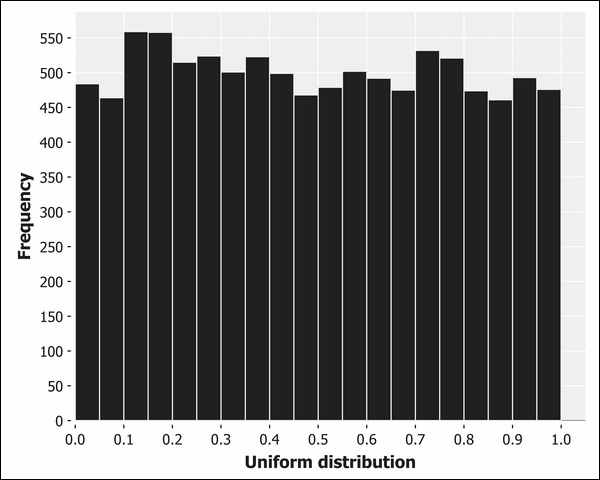
Each bar of the histogram is approximately the same height, corresponding to the equal probability of generating a number that falls into each bin. The bars aren't exactly the same height since the uniform distribution describes the theoretical output that our random sampling can't mirror precisely. Over the next several chapters, we'll learn ways to precisely quantify the difference between theory and practice to determine whether the differences are large enough to be concerned with. In this case, they are not.
If instead we generate a histogram of the means of sequences of numbers, we'll end up with a distribution that looks rather different.
(defn ex-1-16 []
  (let [xs (->> (repeatedly rand)
                (partition 10)
                (map mean)
                (take 10000))]
    (-> (c/histogram xs
                     :x-label "Distribution of means"
                     :nbins 20)
        (i/view))))
The preceding code will provide an output similar to the following histogram:
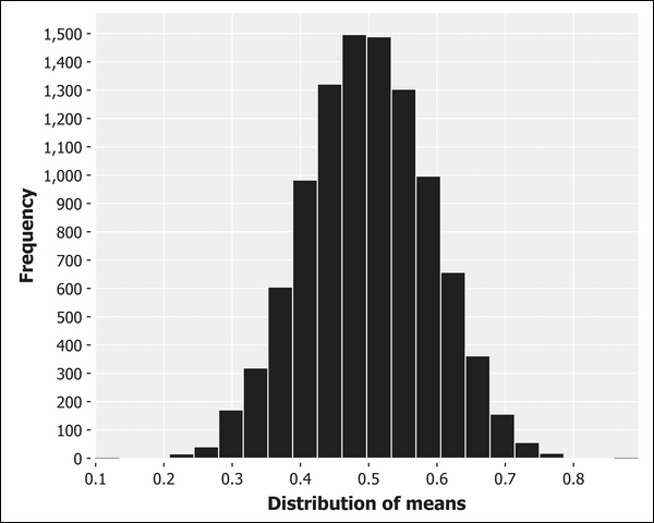
Although it's not impossible for the mean to be close to zero or one, it's exceedingly improbable and grows less probable as both the number of averaged numbers and the number of sampled averages grow. In fact, the output is exceedingly close to the normal distribution.
This outcome—where the average effect of many small random fluctuations leads to the normal distribution—is called the central limit theorem, sometimes abbreviated to CLT, and goes a long way towards explaining why the normal distribution occurs so frequently in natural phenomena.
The central limit theorem wasn't named until the 20th century, although the effect had been documented as early as 1733 by the French mathematician Abraham de Moivre, who used the normal distribution to approximate the number of heads resulting from tosses of a fair coin. The outcome of coin tosses is best modeled with the binomial distribution, which we will introduce in Chapter 4, Classification. While the central limit theorem provides a way to generate samples from an approximate normal distribution, Incanter's distributions namespace provides functions for generating samples efficiently from a variety of distributions, including the normal:
(defn ex-1-17 []
  (let [distribution (d/normal-distribution)
        xs (->> (repeatedly #(d/draw distribution))
                (take 10000))]
    (-> (c/histogram xs
                     :x-label "Normal distribution"
                     :nbins 20)
        (i/view))))
The preceding code generates the following histogram:
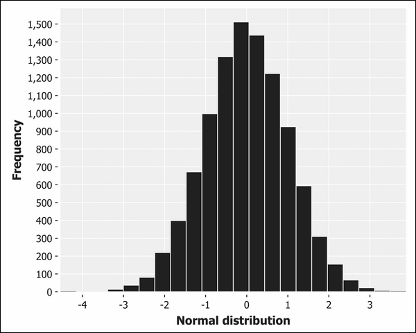
The d/draw function will return one sample from the supplied distribution. The default mean and standard deviation from d/normal-distribution are zero and one respectively.