

Performance measures are used to evaluate learning algorithms and form an important aspect of machine learning. In some cases, these measures are also used as heuristics to build learning models.
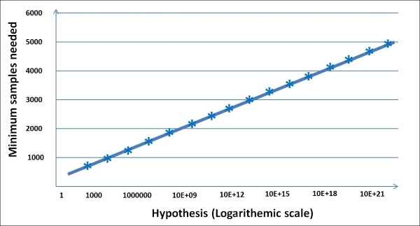
Now let's explore the concept of the Probably Approximately Correct (PAC) theory. While we describe the accuracy of hypothesis, we usually talk about two types of uncertainties as per the PAC theory:
The following graph shows how the number of samples grow with error, probability, and hypothesis:
The error measures for a classification and prediction problem are different. In this section, we will cover some of these error measures followed by how they can be addressed.
In a classification problem, you can have two different types of errors, which can be elegantly represented using the "confusion matrix". Let's say in our target marketing problem, we work on 10,000 customer records to predict which customers are likely to respond to our marketing effort.
After analyzing the campaign, you can construct the following table, where the columns are your predictions and the rows are the real observations:
|
Action |
Predicted (that there will be a buy) |
Predicted (that there will be no buy) |
|---|---|---|
|
Actually bought |
TP: 500 |
FN: 400 |
|
Actually did not buy |
FP: 100 |
TN: 9000 |
In the principal diagonal, we have buyers and non-buyers for whom the prediction matched with reality. These are correct predictions. They are called true positive and true negative respectively. In the upper right-hand side, we have those who we predicted are non-buyers, but in reality are buyers. This is an error known as a false negative error. In the lower left-hand side, we have those we predicted as buyers, but are non-buyers. This is another error known as false positive.
Are both errors equally expensive for the customers? Actually no! If we predict that someone is a buyer and they turn out to be a non-buyer, the company at most would have lost money spent on a mail or a call. However, if we predicted that someone would not buy and they were in fact buyers, the company would not have called them based on this prediction and lost a customer. So, in this case, a false negative is much more expensive than a false positive error.
The Machine learning community uses three different error measures for classification problems:
Measure 1: Accuracy is the percent of predictions that were correct.
Example: The "accuracy" was (9,000+500) out of 10,000 = 95%
Measure 2: Recall is the percent of positives cases that you were able to catch. If false positives are low, recall will be high.
Example: The "recall" was 500 out of 600 = 83.33%
Measure 3: Precision is the percent of positive predictions that were correct. If false negatives are low, precision is high.
Example: The "precision" was 500 out of 900 = 55.55%
In forecasting, you are predicting a continuous variable. So, the error measures are fairly different here. As usual, the error metrics are obtained by comparing the predictions of the models with the real values of the target variables and calculating the average error. Here are a few metrics.
To compute the MSE, we first take the square of the difference between the actual and predicted values of every record. We then take the average value of these squared errors. If the predicted value of the ith record is Pi and the actual value is Ai, then the MSE is:
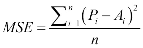
It is also common to use the square root of this quantity called root mean square error (RMSE).
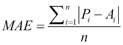
To compute the MAE, we take the absolute difference between the predicted and actual values of every record. We then take the average of those absolute differences. The choice of performance metric depends on the application. The MSE is a good performance metric for many applications as it has more statistical grounding with variance. On the other hand, the MAE is more intuitive and less sensitive to outliers. Looking at the MAE and RMSE gives us additional information about the distribution of the errors. In regression, if the RMSE is close to the MAE, the model makes many relatively small errors. If the RMSE is close to the MAE2, the model makes a few but large errors.
Both the MSE and MAE do not indicate how big the error is as they are numeric values depending on the scale of the target variable. Comparing with a benchmarking index provides a better insight. The common practice is to take the mean of the primary attribute we are predicting and assume that our naïve prediction model is just the mean. Then we compute the MSE based on the naïve model and the original model. The ratio provides an insight into how good or bad our model is compared to the naïve model.
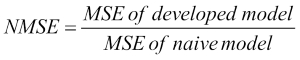
A similar definition can also be used for the MAE.
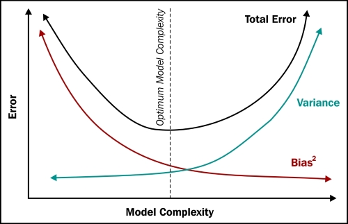
This trap of building highly customized higher order models is called over-fitting and is a critical concept. The resulting error is known as the variance of the model. Essentially, if we had taken a different training set, we would have obtained a very different model. Variance is a measure of the dependency of model on the training set. By the way, the model you see on the right most side (linear fit) is called under-fitting and the error caused due to under-fitting is called bias. In an under-fitting or high bias situation, the model does not explain the relationship between the data. Essentially, we're trying to fit an overly simplistic hypothesis, for example, linear where we should be looking for a higher order polynomial.
To avoid the trap of over-fitting and under-fitting, data scientists build the model on a training set and then find the error on a test set. They refine the model until the error in the test set comes down. As the model starts getting customized to the training data, the error on the test set starts going up. They stop refining the model after that point.
Let's analyze bias and variance a bit more in this chapter and learn a few practical ways of dealing with them. The error in any model can be represented as a combination of bias, variance, and random error. With Err(x)=Bias2+Variance+Irreducible Error in less complex models, the bias term is high, and in models with higher complexity, the variance term is high, as shown in the following figure:
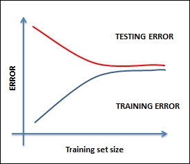
To reduce bias or variance, let's first ask this question. If a model has a high bias, how does its error vary as a function of the amount of data?
At a very low data size, any model can fit the data well (any model fits a single point, any linear model can fit two points, a quadratic can fit three points, and so on). So, the error of a high bias model on a training set starts minuscule and goes up with increasing data points. However, on the test set, the error remains high initially as the model is highly customized to the training set. As the model gets more and more refined, the error reduces and becomes equal to that of the training set.
The following graph depicts the situation clearly:
The remedy for this situation could be one of the following:
Most likely, you are working with very few features, so you must find more features
Increase the complexity of the model by increasing polynomials and depth
Increasing the data size will not be of much help if the model has a high bias

When you face such situations, you can try the following remedies (the reverse of the previous ones):
Most likely, you are working with too many features, so, you must reduce the features
Decrease the complexity of the model
Increasing the data size will be some help