Book Image

Introduction to R for Business Intelligence

By : Jay Gendron
Book Image

Introduction to R for Business Intelligence

By: Jay Gendron

Overview of this book

Explore the world of Business Intelligence through the eyes of an analyst working in a successful and growing company. Learn R through use cases supporting different functions within that company. This book provides data-driven and analytically focused approaches to help you answer questions in operations, marketing, and finance. In Part 1, you will learn about extracting data from different sources, cleaning that data, and exploring its structure. In Part 2, you will explore predictive models and cluster analysis for Business Intelligence and analyze financial times series. Finally, in Part 3, you will learn to communicate results with sharp visualizations and interactive, web-based dashboards. After completing the use cases, you will be able to work with business data in the R programming environment and realize how data science helps make informed decisions and develops business strategy. Along the way, you will find helpful tips about R and Business Intelligence.
Table of Contents (19 chapters)
Introduction to R for Business Intelligence
Credits
About the Author
Acknowledgement
About the Reviewers
www.PacktPub.com
Preface
References
R Packages Used in the Book
R Code for Supporting Market Segment Business Case Calculations

Refining data for simple linear regression


As discussed earlier, there may be times when your diagnostic plots indicate that the data does not meet all the assumptions specified by the LINE approach (Linearity, Independence, Normality, and Equal variance).

Consider the following simple dataset. Run a SLR and generate its diagnostic plots:

x0 <- c(1, 2, 3, 4, 5, 6, 7, 8, 9, 10) 
y0 <- c(1.00, 1.41, 1.73, 2.00, 2.24, 
        2.45, 2.65, 2.83, 3.00, 3.16) 
fit0 <- lm(y0 ~ x0) 
 
par(mfrow = c(1, 3)) 
plot(x0, y0, pch = 19, main = "Linearity?"); abline(fit0) 
hist(fit0$residuals, main = "Normality?", col = "gray") 
plot(fit0$fitted.values, fit0$residuals,  
     main = "Equal Variance?", pch = 19); abline(h = 0) 

The diagnostic plots generated are as follows:

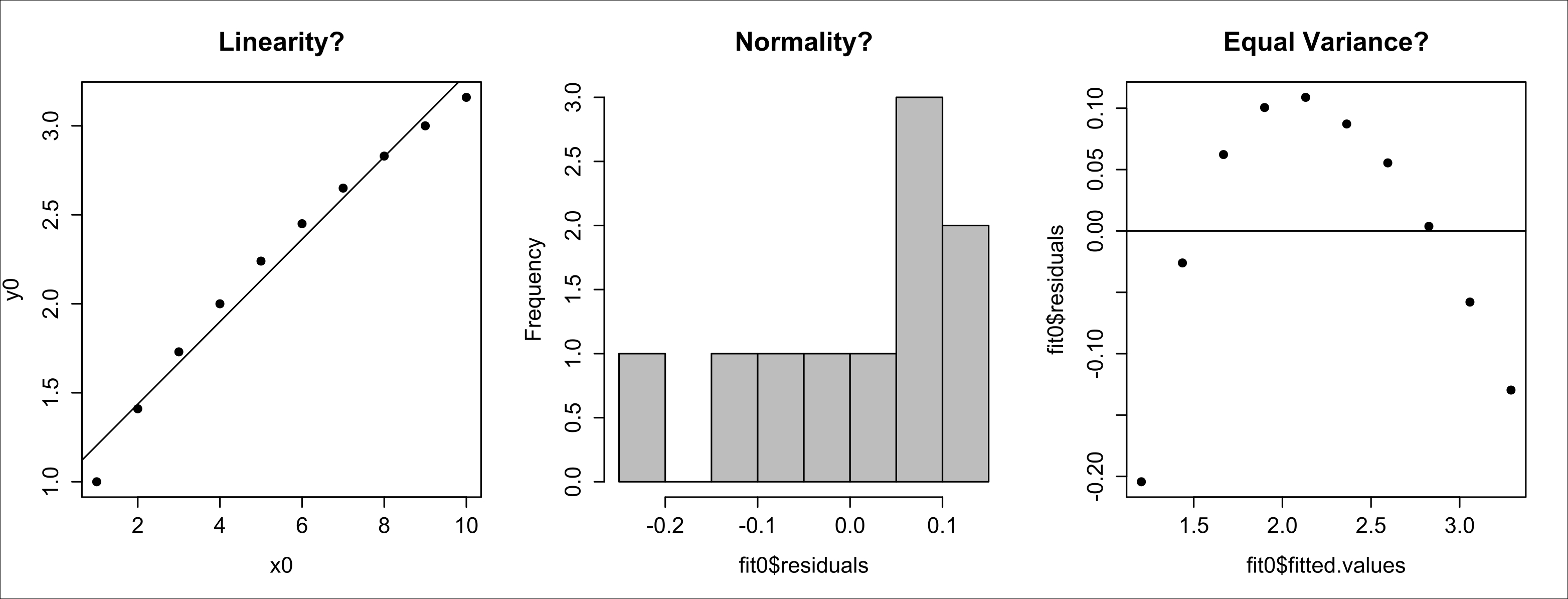
The first plot shows some deviation from linearity. Recall the saying If things look OK, then they probably are OK. You are going to focus on the other two plots, which do not meet the assumptions of normality or equal variance...