The last important concept of this chapter is a behavior known as Amdahl's law. In simple terms, Amdahl's law states that we can parallelize/distribute our computations as much as we want, gaining in performance as we add compute resources. However, our code cannot be faster than the speed of its combined sequential (that is, non parallelizable) parts on a single processor.

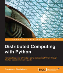
Put more formally, Amdahl's law has the following formulation. Given an algorithm that is partially parallel, let's call P its parallel fraction and S its serial (that is, non parallel) fraction (clearly, S+P=100%). Furthermore, let's call T(n) the runtime (in seconds) of the algorithm when using n processors. Then, the following relation holds:

The preceding relation, translated in plain English states the following:

The execution time of the algorithm described here on n processors is equal—and generally greater—than the execution time of its serial part on one processor (that is, S*T(1)) plus the execution time of its parallel part on one processor (that is, P*T(1)) divided by n: the number of processors.

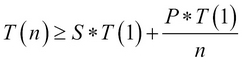
As we increase the number, n, of processors used by our code, the second term on the equation becomes smaller and smaller, eventually becoming negligible with respect to the first term. In those cases, the preceding relation simply becomes this:

The translation of this relation in plain English is as follows:

The execution time of the algorithm described here on an infinite number of processors (that is, a really large number of processors) is approximately equal to the execution time of its serial part on a single processor (that is, S*T(1)).

Now, let's stop for a second and think about the implication of Amdahl's law. What we have here is a pretty simple observation: oftentimes, we cannot fully parallelize our algorithms.

Which means that, most of the time, we cannot have S=0 in the preceding relations. The reasons for this are numerous: we might have to copy data and/or code to where the various processors will be able to access them. We might have to split the data into chunks and move those chunks over the network. We might have to collect the results of all the concurrent tasks and perform some further processing on them, and so on.

Whatever the reason, if we cannot fully parallelize our algorithm, eventually the runtime of our code will be dominated by the performance of the serial fraction. Not only that, but even before that happens, we will start to see increasingly worse-than-expected speedups.

As a side note, algorithms that are fully parallel are usually called embarrassingly parallel or, in a more politically correct way, pleasantly parallel and offer impressive scalability properties (with speedups often linear with the number of processors). Of course, there is nothing embarrassing about those pieces of software! Unfortunately, they are not as common as we would like.

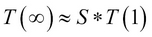
Let's try to visualize the entire Amdahl's law with some numbers. Assume that our algorithm takes 100 seconds on a single processor. Let's also assume that we can parallelize 99% of it, which would be a pretty amazing feat, most of the time. We can make our code go faster by increasing the number of processor we use, as expected. Let's take at look at the following calculation:

We can see from the preceding numbers that the speedup increase with increasing values of n is rather disappointing. We start with a truly amazing 9.2X speedup using 10 processors, and then we drop to just 50X when using 100 processors and a paltry 91X when using 1,000 processors!

The following figure plots the expected best-case speedup for the same algorithm (calculated up to almost n=10,000). It does not matter how many processors we use; we cannot get a speedup greater than 100X, meaning that the fastest our code will run is one second, which is the time its serial fraction takes on a single processor, exactly as predicted by Amdahl's law:

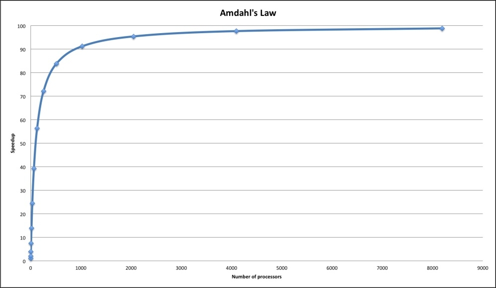
Amdahl's law tells us two things: how much of a speedup we can reasonably expect in the best-case scenario and when to stop throwing hardware at the problem because of diminishing returns.

Another interesting observation is that Amdahl's law applies equally to distributed systems and hybrid parallel-distributed systems as well. In those cases, n refers to the total number of processors across computers.

One aspect that should be mentioned at this point is that as the systems that we can use become more powerful, our distributed algorithms will take less and less time to run, if they can make use of the extra cycles.

When the runtime of our applications becomes reasonably short, what usually happens is that we tend to tackle bigger problems. This aspect of algorithm evolution, namely the expanding of the problem size (and therefore of the computing requirements) once acceptable performance levels are reached, is what is called Gustafson's law.