

Next to speech recognition, there is we can do with sound fragments. While speech recognition focuses on converting speech (spoken words) to digital data, we can also use fragments to identify the person who is speaking. This is also known as voice recognition. Every individual has different characteristics when speaking, caused by differences in anatomy and behavioral patterns. Speaker verification and speaker identification are getting more attention in this digital age. For example, a home digital assistant can automatically detect which person is speaking.
In the following recipe, we'll be using the same data as in the previous recipe, where we implemented a speech recognition pipeline. However, this time, we will be classifying the speakers of the spoken numbers.
- In this recipe, we start by importing all libraries:
import glob
import numpy as np
import random
import librosa
from sklearn.model_selection import train_test_split
from sklearn.preprocessing import LabelBinarizer

import keras
from keras.layers import LSTM, Dense, Dropout, Flatten
from keras.models import Sequential
from keras.optimizers import Adam
from keras.callbacks import EarlyStopping, ModelCheckpoint
- Let's set
SEEDand the location of the.wavfiles:
SEED = 2017
DATA_DIR = 'Data/spoken_numbers_pcm/'
- Let's split the
.wavfiles in a training set and a validation set with scikit-learn'strain_test_splitfunction:
files = glob.glob(DATA_DIR + "*.wav")
X_train, X_val = train_test_split(files, test_size=0.2, random_state=SEED)

print('# Training examples: {}'.format(len(X_train)))
print('# Validation examples: {}'.format(len(X_val)))- To extract and print all unique
labels, we use the following code:
labels = []
for i in range(len(X_train)):
    label = X_train[i].split('/')[-1].split('_')[1]
    if label not in labels:
        labels.append(label)
print(labels)- We can now define our
one_hot_encodefunction as follows:
label_binarizer = LabelBinarizer()
label_binarizer.fit(list(set(labels)))

def one_hot_encode(x): return label_binarizer.transform(x)
- Before we can feed the data to our network, some preprocessing needs to be done. We use the following settings:
n_features = 20
max_length = 80
n_classes = len(labels)
- We can now our batch generator. The generator all preprocessing tasks, such as reading a
.wavfile and transforming it into usable input:
def batch_generator(data, batch_size=16):
    while 1:
        random.shuffle(data)
        X, y = [], []
        for i in range(batch_size):
            wav = data[i]
            wave, sr = librosa.load(wav, mono=True)
            label = wav.split('/')[-1].split('_')[1]
            y.append(one_hot_encode(label))
            mfcc = librosa.feature.mfcc(wave, sr)
            mfcc = np.pad(mfcc, ((0,0), (0, max_length-
            len(mfcc[0]))), mode='constant', constant_values=0)
            X.append(np.array(mfcc))
yield np.array(X), np.array(y)- Let's define the hyperparameters before defining our network architecture:
learning_rate = 0.001
batch_size = 64
n_epochs = 50
dropout = 0.5

input_shape = (n_features, max_length)
steps_per_epoch = 50
- The network architecture we will use is quite straightforward. We will stack an
LSTMlayer on top of a dense layer, as follows:
 model = Sequential()
 model.add(LSTM(256, return_sequences=True, input_shape=input_shape,
   dropout=dropout))
 model.add(Flatten())
 model.add(Dense(128, activation='relu'))
 model.add(Dropout(dropout))
 model.add(Dense(n_classes, activation='softmax'))
- Next, we set the function, compile the model, and a summary of our model:
opt = Adam(lr=learning_rate)
 model.compile(loss='categorical_crossentropy', optimizer=opt,
 metrics=['accuracy'])
 model.summary()
- To prevent overfitting, we will be using early stopping and automatically store the model that has the highest validation accuracy:
callbacks = [ModelCheckpoint('checkpoints/voice_recognition_best_model_{epoch:02d}.hdf5', save_best_only=True),
EarlyStopping(monitor='val_acc', patience=2)]- We are ready to start training and we will store the results in
history:
 history = model.fit_generator(
   generator=batch_generator(X_train, batch_size),
   steps_per_epoch=steps_per_epoch,
   epochs=n_epochs,
   verbose=1,
   validation_data=batch_generator(X_val, 32),
   validation_steps=5,
   callbacks=callbacks
 )
In the following figure, the training accuracy and validation accuracy are plotted against the epochs:
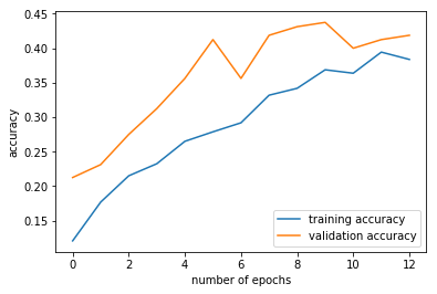
Figure 9.1: Training and validation accuracy