There are many different types of data, such as integer, real number, or string. The following table offers a list of those data types:

In the following examples, we assign a value to r, which is a scalar, and several values to pv, which is an array (vector).The type() function is used to show their types:

>>> import numpy as np
>>> r=0.023
>>>pv=np.array([100,300,500])
>>>type(r)
<class'float'>
>>>type(pv)
<class'numpy.ndarray'>

To choose the appropriate decision, we use the round()function; see the following example:

>>> 7/3
2.3333333333333335
>>>round(7/3,5)
2.33333
>>>

For data manipulation, let's look at some simple operations:

>>>import numpy as np
>>>a=np.zeros(10)                      # array with 10 zeros 
>>>b=np.zeros((3,2),dtype=float)       # 3 by 2 with zeros 
>>>c=np.ones((4,3),float)              # 4 by 3 with all ones 
>>>d=np.array(range(10),float)         # 0,1, 2,3 .. up to 9 
>>>e1=np.identity(4)                   # identity 4 by 4 matrix 
>>>e2=np.eye(4)                        # same as above 
>>>e3=np.eye(4,k=1)                    # 1 start from k 
>>>f=np.arange(1,20,3,float)           # from 1 to 19 interval 3 
>>>g=np.array([[2,2,2],[3,3,3]])       # 2 by 3 
>>>h=np.zeros_like(g)                  # all zeros 
>>>i=np.ones_like(g)                   # all ones

Some so-called dot functions are quite handy and useful:

>>> import numpy as np
>>> x=np.array([10,20,30])
>>>x.sum()
60

Anything after the number sign of # will be a comment. Arrays are another important data type:

>>>import numpy as np
>>>x=np.array([[1,2],[5,6],[7,9]])      # a 3 by 2 array
>>>y=x.flatten()
>>>x2=np.reshape(y,[2,3]              ) # a 2 by 3 array

We could assign a string to a variable:

>>> t="This is great"
>>>t.upper()
'THIS IS GREAT'
>>>

To find out all string-related functions, we use dir(''); see the following code:

>>>dir('')
['__add__', '__class__', '__contains__', '__delattr__', '__dir__', '__doc__', '__eq__', '__format__', '__ge__', '__getattribute__', '__getitem__', '__getnewargs__', '__gt__', '__hash__', '__init__', '__iter__', '__le__', '__len__', '__lt__', '__mod__', '__mul__', '__ne__', '__new__', '__reduce__', '__reduce_ex__', '__repr__', '__rmod__', '__rmul__', '__setattr__', '__sizeof__', '__str__', '__subclasshook__', 'capitalize', 'casefold', 'center', 'count', 'encode', 'endswith', 'expandtabs', 'find', 'format', 'format_map', 'index', 'isalnum', 'isalpha', 'isdecimal', 'isdigit', 'isidentifier', 'islower', 'isnumeric', 'isprintable', 'isspace', 'istitle', 'isupper', 'join', 'ljust', 'lower', 'lstrip', 'maketrans', 'partition', 'replace', 'rfind', 'rindex', 'rjust', 'rpartition', 'rsplit', 'rstrip', 'split', 'splitlines', 'startswith', 'strip', 'swapcase', 'title', 'translate', 'upper', 'zfill']
>>>

For example, from the preceding list we see a function called split. After typinghelp(''.split), we will have related help information:

>>>help(''.split)
Help on built-in function split:

split(...) method of builtins.str instance
S.split(sep=None, maxsplit=-1) -> list of strings

    Return a list of the words in S, using sep as the
delimiter string. If maxsplit is given, at most maxsplit
splits are done. If sep is not specified or is None, any
whitespace string is a separator and empty strings are
removed from the result.
>>>

We could try the following example:

>>> x="this is great"
>>>x.split()
['this', 'is', 'great']
>>>

Matrix manipulation is important when we deal with various matrices:

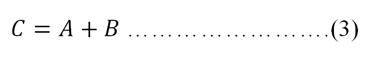
The condition for equation (3) is that matrices A and B should have the same dimensions. For the product of two matrices, we have the following equation:

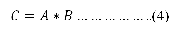
Here,A is an n by k matrix (n rows and k columns), while B is a k by m matrix. Remember that the second dimension of the first matrix should be the same as the first dimension of the second matrix. In this case, it is k. If we assume that the individual data items in C, A, and B are Ci,j (the ith row and the jth column), Ai,j, and Bi,j, we have the following relationship between them:

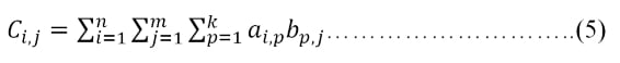
The dot() function from the NumPy module could be used to carry the preceding matrix multiplication:

>>>a=np.array([[1,2,3],[4,5,6]],float)    # 2 by 3
>>>b=np.array([[1,2],[3,3],[4,5]],float)  # 3 by 2
>>>np.dot(a,b)                            # 2 by 2
>>>print(np.dot(a,b))
array([[ 19.,  23.],
[ 43.,  53.]])
>>>

We could manually calculate c(1,1): 1*1 + 2*3 + 3*4=19.

After retrieving data or downloading data from the internet, we need to process it. Such a skill to process various types of raw data is vital to finance students and to professionals working in the finance industry. Here we will see how to download price data and then estimate returns.

Assume that we have n values of x1, x2, … and xn. There exist two types of means: arithmetic mean and geometric mean; see their genetic definitions here:

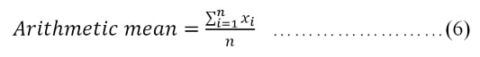
Assume that there exist three values of 2,3, and 4. Their arithmetic and geometric means are calculated here:

>>>(2+3+4)/3.
>>>3.0
>>>geo_mean=(2*3*4)**(1./3)
>>>round(geo_mean,4) 
2.8845

For returns, the arithmetic mean's definition remains the same, while the geometric mean of returns is defined differently; see the following equations:

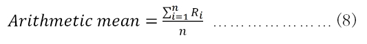
In Chapter 3, Time Value of Money, we will discuss both means again.

We could say that NumPy is a basic module while SciPy is a more advanced one. NumPy tries to retain all features supported by either of its predecessors, while most new features belong in SciPy rather than NumPy. On the other hand, NumPy and SciPy have many overlapping features in terms of functions for finance. For those two types of definitions, see the following example:

>>> import scipy as sp
>>> ret=sp.array([0.1,0.05,-0.02])
>>>sp.mean(ret)
0.043333333333333342
>>>pow(sp.prod(ret+1),1./len(ret))-1 
0.042163887067679262

Our second example is related to processing theFama-French 3 factor time series. Since this example is more complex than the previous one, if a user feels it is difficult to understand, he/she could simply skip this example. First, a ZIP file called F-F_Research_Data_Factor_TXT.zip could be downloaded from Prof. French's Data Library. After unzipping and removing the first few lines and annual datasets, we will have a monthly Fama-French factor time series. The first few lines and last few lines are shown here:

DATE    MKT_RFSMBHMLRF
192607    2.96   -2.30   -2.87    0.22
192608    2.64   -1.40    4.19    0.25
192609    0.36   -1.32    0.01    0.23

201607    3.95    2.90   -0.98    0.02
201608    0.49    0.94    3.18    0.02
201609    0.25    2.00   -1.34    0.02

Assume that the final file is called ffMonthly.txt under c:/temp/. The following program is used to retrieve and process the data:

import numpy as np
import pandas as pd
file=open("c:/temp/ffMonthly.txt","r")
data=file.readlines()
f=[]
index=[]
for i in range(1,np.size(data)):
    t=data[i].split()
    index.append(int(t[0]))
    for j in range(1,5):
        k=float(t[j])
        f.append(k/100)
n=len(f) 
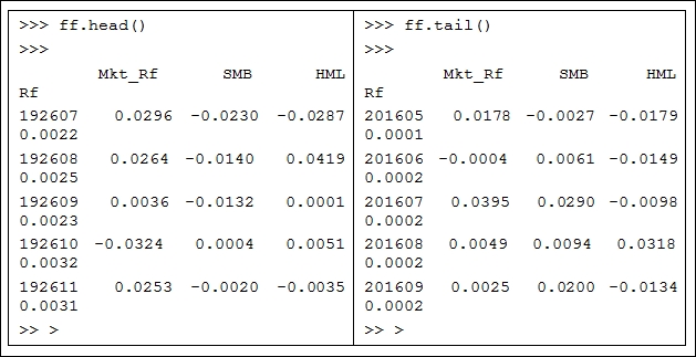
f1=np.reshape(f,[n/4,4])
ff=pd.DataFrame(f1,index=index,columns=['Mkt_Rf','SMB','HML','Rf'])

To view the first and last few observations for the dataset called ff, the functions of .head() and .tail()can be used: