The zero-mean models have a constant mean and constant variance and shows no predictable trends or seasonality. Observations from a zero mean model are assumed to be independent and identically distributed (iid) and represent the random noise around a fixed mean, which has been deducted from the time series as a constant term.

Let us consider that X₁, X₂, ... ,X_n represent the random variables corresponding to n observations of a zero mean model. If x₁, x₂, ... ,x_n are n observations from the zero mean time series, then the joint distribution of the observations is given as a product of probability mass function for every time index as follows:

P(X1 = x1,X2 = x2 , ... , Xn = xn) = f(X1 = x1) f(X2 = x2) ... f(Xn = xn)

Most commonly f(X_t = x_t) is modeled by a normal distribution of mean zero and variance σ ², which is assumed to be the irreducible error of the model and hence treated as a random noise. The following figure shows a zero-mean series of normally distributed random noise of unit variance:

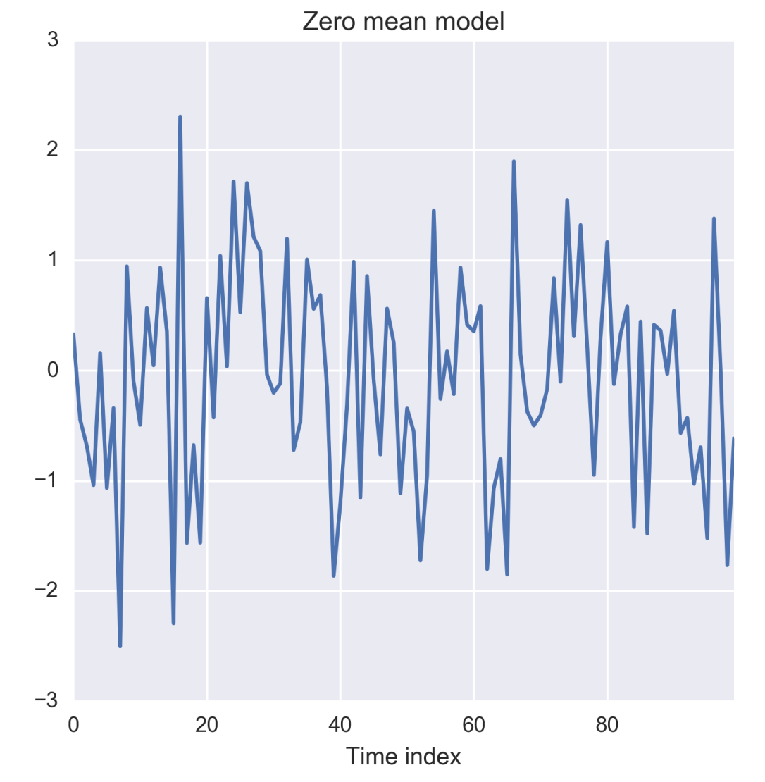
Figure 1.12: Zero-mean time series

The preceding plot is generated by the following code:

import os 
import numpy as np 
%matplotlib inline 
from matplotlib import pyplot as plt 
import seaborn as sns 
os.chdir('D:/Practical Time Series/') 
zero_mean_series = np.random.normal(loc=0.0, scale=1., size=100) 

The zero mean with constant variance represents a random noise that can assume infinitely possible real values and is suited for representing irregular variations in the time series of a continuous variable. However in many cases, the observable state of the system or process might be discrete in nature and confined to a finite number of possible values s₁,s₂, ... , s_m. In such cases, the observed variable (X) is assumed to obey the multinomial distribution, P(X = s₁ )= p₁, P(X = s₂ ) = p₂,…,P(X = s_m) = p_m such that p₁ + p₂ + ... + p_m = 1. Such a time series is a discrete stochastic process.

Multiple throws a dice over time is an example of a discrete stochastic process with six possible outcomes for any throw. A simpler discrete stochastic process is a binary process such as tossing a coin such as only two outcomes namely head and tail. The following figure shows 100 runs from a simulated process of throwing a biased dice for which probability of turning up an even face is higher than that of showing an odd face. Note the higher number of occurrences of even faces, on an average, compared to the number of occurrences of odd faces.

A random walk is given as a sum of n iids, which has zero mean and constant variance. Based on this definition, the realization of a random walk at time index t is given by the sum S = x₁ + x₂ + ... + x_n. The following figure shows the random walk obtained from iids, which vary according to a normal distribution of zero mean and unit variance.

The random walk is important because if such behavior is found in a time series, it can be easily reduced to zero mean model by taking differences of the observations from two consecutive time indices as S_t - S_t-1 = x_t is an iid with zero mean and constant variance.

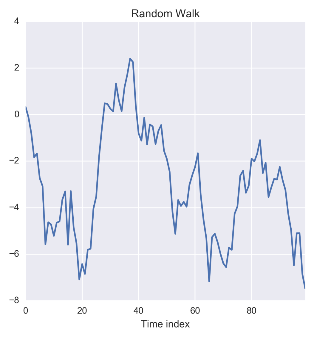
Figure 1.13: Random walk time series

The random walk in the preceding figure can be generated by taking the cumulative sum of the zero mean model discussed in the previous section. The following code implements this:

random_walk = np.cumsum(zero_mean_series) 
plt.figure(figsize=(5.5, 5.5)) 
g = sns.tsplot(random_walk) 
g.set_title('Random Walk') 
g.set_xlabel('Time index') 

This type of model aims to capture the long run trend in the time series that can be fitted as linear regression of the time index. When the time series does not exhibit any periodic or seasonal fluctuations, it can be expressed just as the sum of the trend and the zero mean model as x_t = μ(t) + y_t, where μ(t) is the time-dependent long run trend of the series.

The choice of the trend model μ(t) is critical to correctly capturing the behavior of the time series. Exploratory data analysis often provides hints for hypothesizing whether the model should be linear or non-linear in t. A linear model is simply μ(t) = wt + b, whereas quadratic model is μ(t) = w₁t + w₂t² + b. Sometimes, the trend can be hypothesized by a more complex relationship in terms of the time index such as μ(t) = w₀t^p + b.

The weights and biases in the trend modes such as the ones discussed previously is obtained by running a regression with t as the explanatory variable and μ as the explained. The residuals x_t - μ(t) of the trend model is considered to the irreducible noise and as realization of the zero mean component y_t.

Seasonality manifests as periodic and repetitive fluctuations in a time series and hence are modelled as sum of weighted sum of sine waves of known periodicity. Assuming that long run trend has been removed by a trend line, the seasonality model can be expressed as x_t = s_t + y_t, where the seasonal variation

Seasonality models are also known as harmonic regression model as they attempt to fit the sum of multiple sin waves.

The four models described here are building blocks of a fully-fledged time series model. As you might have gathered by now, a zero sum model represents irreducible error of the system and all of other three models aim to transform a given time series to the zero sum models through suitable mathematical transformations. To get forecasts in terms of the original time series, relevant inverse transformations are applied.

The upcoming chapters detail the four models discussed here. However, we have reached a point where we can summarize the generic approach of a time series analysis in the following four steps:

These steps are most commonly enough to develop mathematical models for most time series. The individual trend and seasonality models can be simple or complex depending on the original time series and the application.