We will study AdamOptimizer here; TensorFlow AdamOptimizer uses Kingma and Ba's Adam algorithm to manage the learning rate. Adam has many advantages over the simple GradientDescentOptimizer. The first is that it uses moving averages of the parameters, which enables Adam to use a larger step size, and it will converge to this step size without any fine-tuning.

The disadvantage of Adam is that it requires more computation to be performed for each parameter in each training step. GradientDescentOptimizer can be used as well, but it would require more hyperparameter tuning before it would converge as quickly. The following example shows how to use AdamOptimizer:

Here, automatic differentiation computes gradients without user input:

import numpy as np
import seaborn
import matplotlib.pyplot as plt
import tensorflow as tf

# input dataset
xData = np.arange(100, step=.1)
yData = xData + 20 * np.sin(xData/10)

# scatter plot for input data
plt.scatter(xData, yData)
plt.show()

# defining data size and batch size
nSamples = 1000
batchSize = 100

# resize
xData = np.reshape(xData, (nSamples,1))
yData = np.reshape(yData, (nSamples,1))

# input placeholders
x = tf.placeholder(tf.float32, shape=(batchSize, 1))
y = tf.placeholder(tf.float32, shape=(batchSize, 1))

# init weight and bias
with tf.variable_scope("linearRegression"):
 W = tf.get_variable("weights", (1, 1), initializer=tf.random_normal_initializer())
 b = tf.get_variable("bias", (1,), initializer=tf.constant_initializer(0.0))

 y_pred = tf.matmul(x, W) + b
 loss = tf.reduce_sum((y - y_pred)**2/nSamples)

# optimizer
opt = tf.train.AdamOptimizer().minimize(loss)
with tf.Session() as sess:
    sess.run(tf.global_variables_initializer())

    # gradient descent loop for 500 steps
    for _ in range(500):
     # random minibatch
     indices = np.random.choice(nSamples, batchSize)

     X_batch, y_batch = xData[indices], yData[indices]

     # gradient descent step
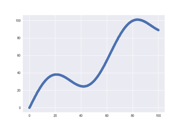
     _, loss_val = sess.run([opt, loss], feed_dict={x: X_batch, y: y_batch})

Here is the scatter plot for the dataset:

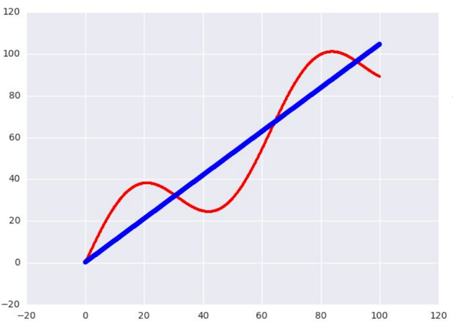
This is the plot of the learned model on the data: