

Machine learning algorithms work with data. They create associations, find out relationships, discover patterns, generate new samples, and more, working with well-defined datasets. Unfortunately, sometimes the assumptions or the conditions imposed on them are not clear, and a lengthy training process can result in a complete validation failure. Even if this condition is stronger in deep learning contexts, we can think of a model as a gray box (some transparency is guaranteed by the simplicity of many common algorithms), where a vectorial input

is transformed into a vectorial output

:
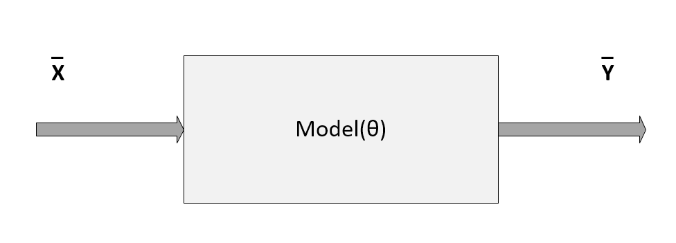
Schema of a generic model parameterized with the vector θ
In the previous diagram, the model has been represented by a pseudo-function that depends on a set of parameters defined by the vector θ. In this section, we are only considering parametric models, although there's a family of algorithms that are called non-parametric, because they are based only on the structure of the data. We're going to discuss some of them in upcoming chapters.
The task of a parametric learning process is therefore to find the best parameter set that maximizes a target function whose value is proportional to the accuracy (or the error, if we are trying to minimize them) of the model given a specific input X and output Y. This definition is not very rigorous, and it will be improved in the following sections; however, it's useful as a way to understand the context we're working in.
Then, the first question to ask is: What is the nature of X? A machine learning problem is focused on learning abstract relationships that allow a consistent generalization when new samples are provided. More specifically, we can define a stochastic data generating process with an associated joint probability distribution:

Sometimes, it's useful to express the joint probability p(x, y) as a product of the conditional p(y|x), which expresses the probability of a label given a sample, and the marginal probability of the samples p(x). This expression is particularly useful when the prior probability p(x) is known in semi-supervised contexts, or when we are interested in solving problems using the Expectation Maximization (EM) algorithm. We're going to discuss this approach in upcoming chapters.
In many cases, we are not able to derive a precise distribution; however, when considering a dataset, we always assume that it's drawn from the original data-generating distribution. This condition isn't a purely theoretical assumption, because, as we're going to see, whenever our data points are drawn from different distributions, the accuracy of the model can dramatically decrease.
If we sample N independent and identically distributed (i.i.d.) values from pdata, we can create a finite dataset X made up of k-dimensional real vectors:

In a supervised scenario, we also need the corresponding labels (with t output values):

When the output has more than two classes, there are different possible strategies to manage the problem. In classical machine learning, one of the most common approaches is One-vs-All, which is based on training N different binary classifiers where each label is evaluated against all the remaining ones. In this way, N-1 is performed to determine the right class. With shallow and deep neural networks, instead, it's preferable to use a softmax function to represent the output probability distribution for all classes:

This kind of output (zi represents the intermediate values, and the sum of the terms is normalized to 1) can be easily managed using the cross-entropy cost function (see the corresponding paragraph in the Loss and cost functions section).
Many algorithms show better performances (above all, in terms of training speed) when the dataset is symmetric (with a zero-mean). Therefore, one of the most important preprocessing steps is so-called zero-centering, which consists in subtracting the feature-wise mean Ex[X] from all samples:

This operation, if necessary, is normally reversible, and doesn't alter relationships both among samples and among components of the same sample. In deep learning scenarios, a zero-centered dataset allows exploiting the symmetry of some activation function, driving to a faster convergence (we're going to discuss these details in the next chapters).
Another very important preprocessing step is called whitening, which is the operation of imposing an identity covariance matrix to a zero-centered dataset:

As the covariance matrix Ex[XTX] is real and symmetric, it's possible to eigendecompose it without the need to invert the eigenvector matrix:

The matrix V contains the eigenvectors (as columns), and the diagonal matrix Ω contains the eigenvalues. To solve the problem, we need to find a matrix A, such that:

Using the eigendecomposition previously computed, we get:

Hence, the matrix A is:

One of the main advantages of whitening is the decorrelation of the dataset, which allows an easier separation of the components. Furthermore, if X is whitened, any orthogonal transformation induced by the matrix P is also whitened:

Moreover, many algorithms that need to estimate parameters that are strictly related to the input covariance matrix can benefit from this condition, because it reduces the actual number of independent variables (in general, these algorithms work with matrices that become symmetric after applying the whitening). Another important advantage in the field of deep learning is that the gradients are often higher around the origin, and decrease in those areas where the activation functions (for example, the hyperbolic tangent or the sigmoid) saturate (|x| → ∞). That's why the convergence is generally faster for whitened (and zero-centered) datasets.
In the following graph, it's possible to compare an original dataset,zero-centering, and whitening:
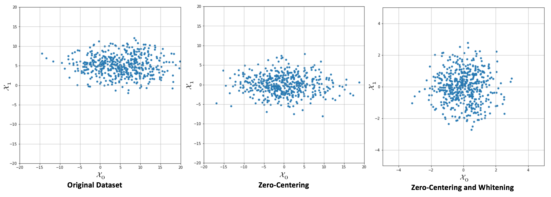
Original dataset (left), centered version (center), whitened version (right)
When a whitening is needed, it's important to consider some important details. The first one is that there's a scale difference between the real sample covariance and the estimation XTX, often adopted with the singular value decomposition (SVD). The second one concerns some common classes implemented by many frameworks, like Scikit-Learn's StandardScaler. In fact, while zero-centering is a feature-wise operation, a whitening filter needs to be computed considering the whole covariance matrix (StandardScaler implements only unit variance, feature-wise scaling).
Luckily, all Scikit-Learn algorithms that benefit from or need a whitening preprocessing step provide a built-in feature, so no further actions are normally required; however, for all readers who want to implement some algorithms directly, I've written two Python functions that can be used both for zero-centering and whitening. They assume a matrix X with a shape (NSamples × n). Moreover, the whiten() function accepts the parameter correct, which allows us to apply the scaling correction (the default value is True):
import numpy as np

def zero_center(X):
    return X - np.mean(X, axis=0)

def whiten(X, correct=True):
    Xc = zero_center(X)
    _, L, V = np.linalg.svd(Xc)
    W = np.dot(V.T, np.diag(1.0 / L))
return np.dot(Xc, W) * np.sqrt(X.shape[0]) if correct else 1.0In real problems, the number of samples is limited, and it's usually necessary to split the initial set X (together with Y) into two subsets as follows:
According to the nature of the problem, it's possible to choose a split percentage ratio of 70% – 30% (a good practice in machine learning, where the datasets are relatively small), or a higher training percentage (80%, 90%, up to 99%) for deep learning tasks where the number of samples is very high. In both cases, we are assuming that the training set contains all the information required for a consistent generalization. In many simple cases, this is true and can be easily verified; but with more complex datasets, the problem becomes harder. Even if we think to draw all the samples from the same distribution, it can happen that a randomly selected test set contains features that are not present in other training samples. Such a condition can have a very negative impact on global accuracy and, without other methods, it can also be very difficult to identify. This is one of the reasons why, in deep learning, training sets are huge: considering the complexity of the features and structure of the data generating distributions, choosing large test sets can limit the possibility of learning particular associations.
In Scikit-Learn, it's possible to split the original dataset using the train_test_split() function, which allows specifying the train/test size, and if we expect to have randomly shuffled sets (default). For example, if we want to split X and Y, with 70% training and 30% test, we can use:
from sklearn.model_selection import train_test_split

X_train, X_test, Y_train, Y_test = train_test_split(X, Y, train_size=0.7, random_state=1)
Shuffling the sets is always a good practice, in order to reduce the correlation between samples. In fact, we have assumed that X is made up of i.i.d samples, but several times two subsequent samples have a strong correlation, reducing the training performance. In some cases, it's also useful to re-shuffle the training set after each training epoch; however, in the majority of our examples, we are going to work with the same shuffled dataset throughout the whole process. Shuffling has to be avoided when working with sequences and models with memory: in all those cases, we need to exploit the existing correlation to determine how the future samples are distributed.
Note
When working with NumPy and Scikit-Learn, it's always a good practice to set the random seed to a constant value, so as to allow other people to reproduce the experiment with the same initial conditions. This can be achieved by calling np.random.seed(...) and using the random-state parameter present in many Scikit-Learn methods.
A valid method to detect the problem of wrongly selected test sets is provided by the cross-validation technique. In particular, we're going to use the K-Fold cross-validation approach. The idea is to split the whole dataset X into a moving test set and a training set (the remaining part). The size of the test set is determined by the number of folds so that, during k iterations, the test set covers the whole original dataset.
In the following diagram, we see a schematic representation of the process:
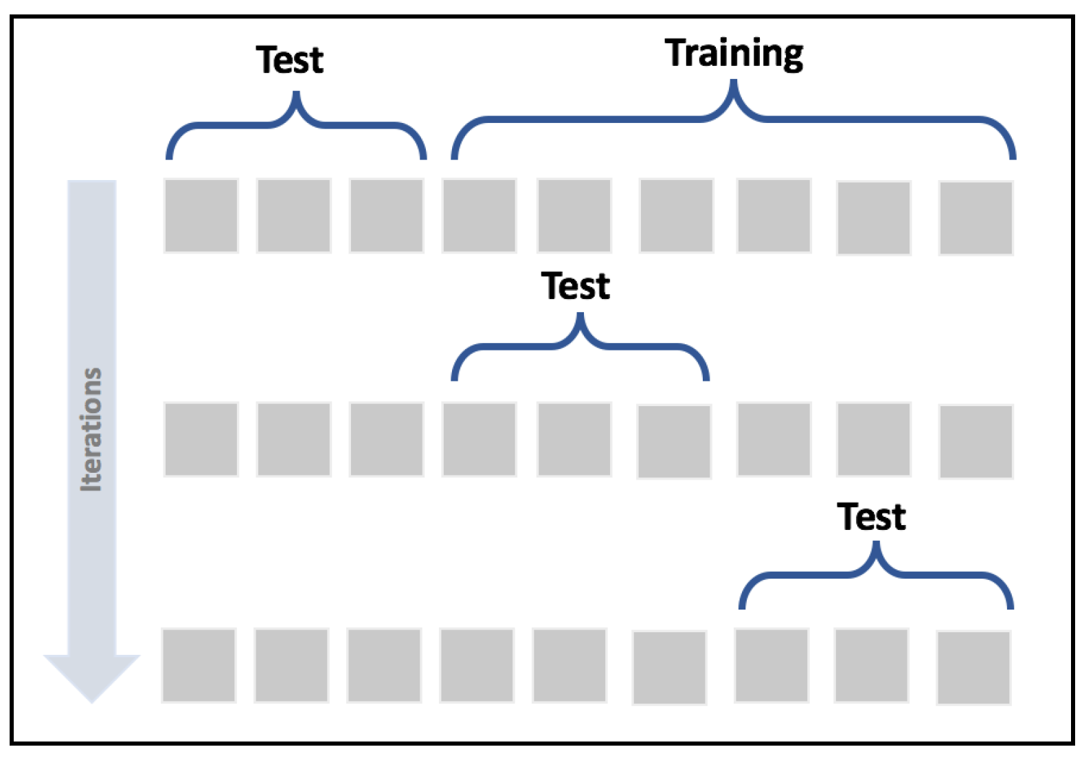
K-Fold cross-validation schema
In this way, it's possible to assess the accuracy of the model using different sampling splits, and the training process can be performed on larger datasets; in particular, on (k-1)*N samples. In an ideal scenario, the accuracy should be very similar in all iterations; but in most real cases, the accuracy is quite below average. This means that the training set has been built excluding samples that contain features necessary to let the model fit the separating hypersurface considering the real pdata. We're going to discuss these problems later in this chapter; however, if the standard deviation of the accuracies is too high (a threshold must be set according to the nature of the problem/model), that probably means that X hasn't been drawn uniformly from pdata, and it's useful to evaluate the impact of the outliers in a preprocessing stage. In the following graph, we see the plot of a 15-fold cross-validation performed on a logistic regression:
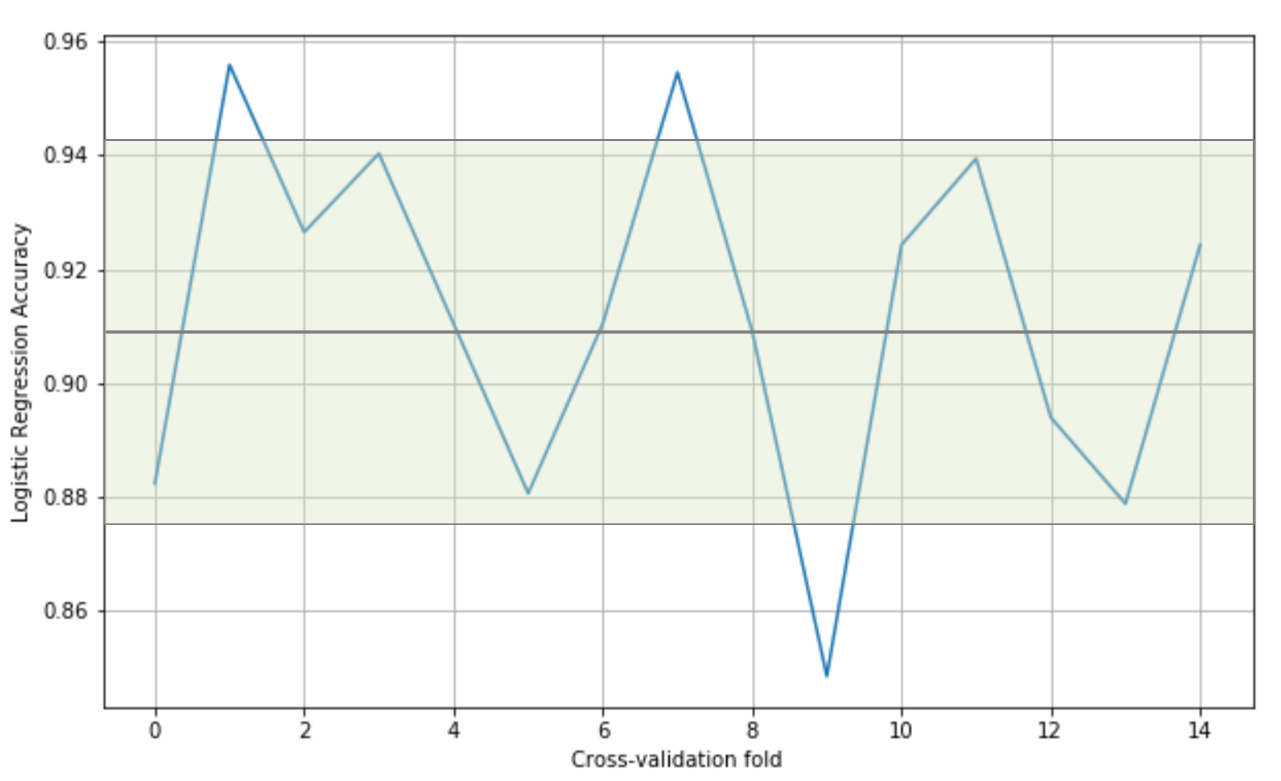
Cross-validation accuracies
The values oscillate from 0.84 to 0.95, with an average (solid horizontal line) of 0.91. In this particular case, considering the initial purpose was to use a linear classifier, we can say that all folds yield high accuracies, confirming that the dataset is linearly separable; however, there are some samples (excluded in the ninth fold) that are necessary to achieve a minimum accuracy of about 0.88.
K-Fold cross-validation has different variants that can be employed to solve specific problems:
- Leave-one-out (LOO): This approach is the most drastic because it creates N folds, each of them containing N-1 training samples and only 1 test sample. In this way, the maximum possible number of samples is used for training, and it's quite easy to detect whether the algorithm is able to learn with sufficient accuracy, or if it's better to adopt another strategy. The main drawback of this method is that N models must be trained, and when N is very large this can cause a performance issue. Moreover, with a large number of samples, the probability that two random values are similar increases, therefore many folds will yield almost identical results. At the same time, LOO limits the possibilities for assessing the generalization ability, because a single test sample is not enough for a reasonable estimation.
- Leave-P-out (LPO): In this case, the number of test samples is set to p (non-disjoint sets), so the number of folds is equal to the binomial coefficient of n over p. This approach mitigates LOO's drawbacks, and it's a trade-off between K-Fold and LOO. The number of folds can be very high, but it's possible to control it by adjusting the number p of test samples; however, if p isn't small or big enough, the binomial coefficient can explode. In fact, when p has about n/2 samples, the number of folds is maximal:

Scikit-Learn implements all those methods (with some other variations), but I suggest always using the cross_val_score() function, which is a helper that allows applying the different methods to a specific problem. In the following snippet based on a polynomial Support Vector Machine (SVM) and the MNIST digits dataset, the function is applied specifying the number of folds (parameter cv). In this way, Scikit-Learn will automatically use Stratified K-Fold for categorical classifications, and Standard K-Fold for all other cases:
from sklearn.datasets import load_digits
from sklearn.model_selection import cross_val_score
from sklearn.svm import SVC

data = load_digits()
svm = SVC(kernel='poly')

skf_scores = cross_val_score(svm, data['data'], data['target'], cv=10)

print(skf_scores)
[ 0.96216216  1.          0.93922652  0.99444444  0.98882682  0.98882682
  0.99441341  0.99438202  0.96045198  0.96590909]

print(skf_scores.mean())
0.978864325583
The accuracy is very high (> 0.9) in every fold, therefore we expect to have even higher accuracy using the LOO method. As we have 1,797 samples, we expect the same number of accuracies:
from sklearn.model_selection import cross_val_score, LeaveOneOut

loo_scores = cross_val_score(svm, data['data'], data['target'], cv=LeaveOneOut())

print(loo_scores[0:100])
[ 1.  1.  1.  1.  1.  0.  1.  1.  1.  1.  1.  1.  1.  1.  1.  1.  1.  1.
  1.  1.  1.  1.  1.  1.  1.  1.  1.  1.  1.  1.  1.  1.  1.  1.  1.  1.
  1.  0.  1.  1.  1.  1.  1.  1.  1.  1.  1.  1.  1.  1.  1.  1.  1.  1.
  1.  1.  1.  1.  1.  1.  1.  1.  1.  1.  1.  1.  1.  1.  1.  0.  1.  1.
  1.  1.  1.  1.  1.  1.  1.  1.  1.  1.  1.  1.  1.  1.  1.  1.  1.  1.
  1.  1.  1.  1.  1.  1.  1.  1.  1.  1.]

print(loo_scores.mean())
0.988870339455
As expected, the average score is very high, but there are still samples that are misclassified. As we're going to discuss, this situation could be a potential candidate for overfitting, meaning that the model is learning perfectly how to map the training set, but it's losing its ability to generalize; however, LOO is not a good method to measure this model ability, due to the size of the validation set.
We can now evaluate our algorithm with the LPO technique. Considering what was explained before, we have selected the smaller Iris dataset and a classification based on a logistic regression. As there are N=150 samples, choosing p = 3, we get 551,300 folds:
from sklearn.datasets import load_iris
from sklearn.linear_model import LogisticRegression
from sklearn.model_selection import cross_val_score, LeavePOut

data = load_iris()

p = 3
lr = LogisticRegression()

lpo_scores = cross_val_score(lr, data['data'], data['target'], cv=LeavePOut(p))

print(lpo_scores[0:100])
[ 1.          1.          1.          1.          1.          1.          1.
  1.          1.          1.          1.          1.          1.          1.
  1.          1.          1.          1.          1.          1.          1.
  1.          1.          1.          1.          1.          1.          1.
  1.          1.          1.          1.          1.          1.          1.
  1.          1.          1.          1.          1.          1.          1.
  1.          1.          1.          1.          1.          1.          1.
  1.          1.          1.          1.          1.          1.          1.
  1.          1.          1.          1.          1.          1.          1.
  1.          0.66666667  ...

print(lpo_scores.mean())
0.955668420098
As in the previous example, we have printed only the first 100 accuracies; however, the global trend can be immediately understood with only a few values.
The cross-validation technique is a powerful tool that is particularly useful when the performance cost is not too high. Unfortunately, it's not the best choice for deep learning models, where the datasets are very large and the training processes can take even days to complete. However, as we're going to discuss, in those cases the right choice (the split percentage), together with an accurate analysis of the datasets and the employment of techniques such as normalization and regularization, allows fitting models that show an excellent generalization ability.