The word regression sounds like go back in some ways. If you've been trying to quit smoking but then yield to the desire to have a cigarette again, you are experiencing an episode of regression. The term regression has appeared in early writings since the late 1300s, and is derived from the Latin term regressus, which means a return. It is used in different fields with different meanings, but in any case, it is always referred to as the action of regressing.

In philosophy, regression is used to indicate the inverse logical procedure with respect to that of the normal apodictic (apodixis), in which we proceed from the general to the particular. Whereas in reality, in regression we go back from the particular to the general, from the effect to the cause, from the conditioned to the condition. In this way, we can draw completely general conclusions from a particular case. This is the first form of generalization that, as we will see later, represents a crucial part of a statistical analysis.

For example, there is marine regression, which is a geological process that occurs as a result of areas of submerged seafloor being exposed more than the sea level. And there is the opposite event, marine transgression; it occurs when flooding from the sea submerges land that was previously exposed.

The following image shows the results of marine regression on the Aral lake.  This lake lies between Kazakhstan and Uzbekistan and has been steadily shrinking since the 1960s, after the rivers that fed it were diverted by Soviet irrigation projects. By 1997, it had declined to ten percent of its original size:

However, in statistics, regression is related to the study of the relationship between the explanatory variables and the response variable. Don't worry! This is the topic we will discuss in this book.

In statistics, the term regression has an ancient origin and a very special meaning. The man who coined this term was a certain Francis Galton, geneticist, who in 1889 published an article in which he demonstrated how every characteristic of an individual is inherited by their offspring, but on an average to a lesser degree. For example, children with tall parents are also tall, but on an average their height will be comparatively less than that of their parents. This phenomenon, also graphically described, is called regression. Since then, this term has lived on to define statistical techniques that analyze relationships between two or more variables.

The following table shows a short summary of the data used by Galton for his study:

Galton depicted in a chart the average height of the parents and that of the children, noting what he called regression in the data.

The following figure shows this data and a regression line that confirms his thesis:

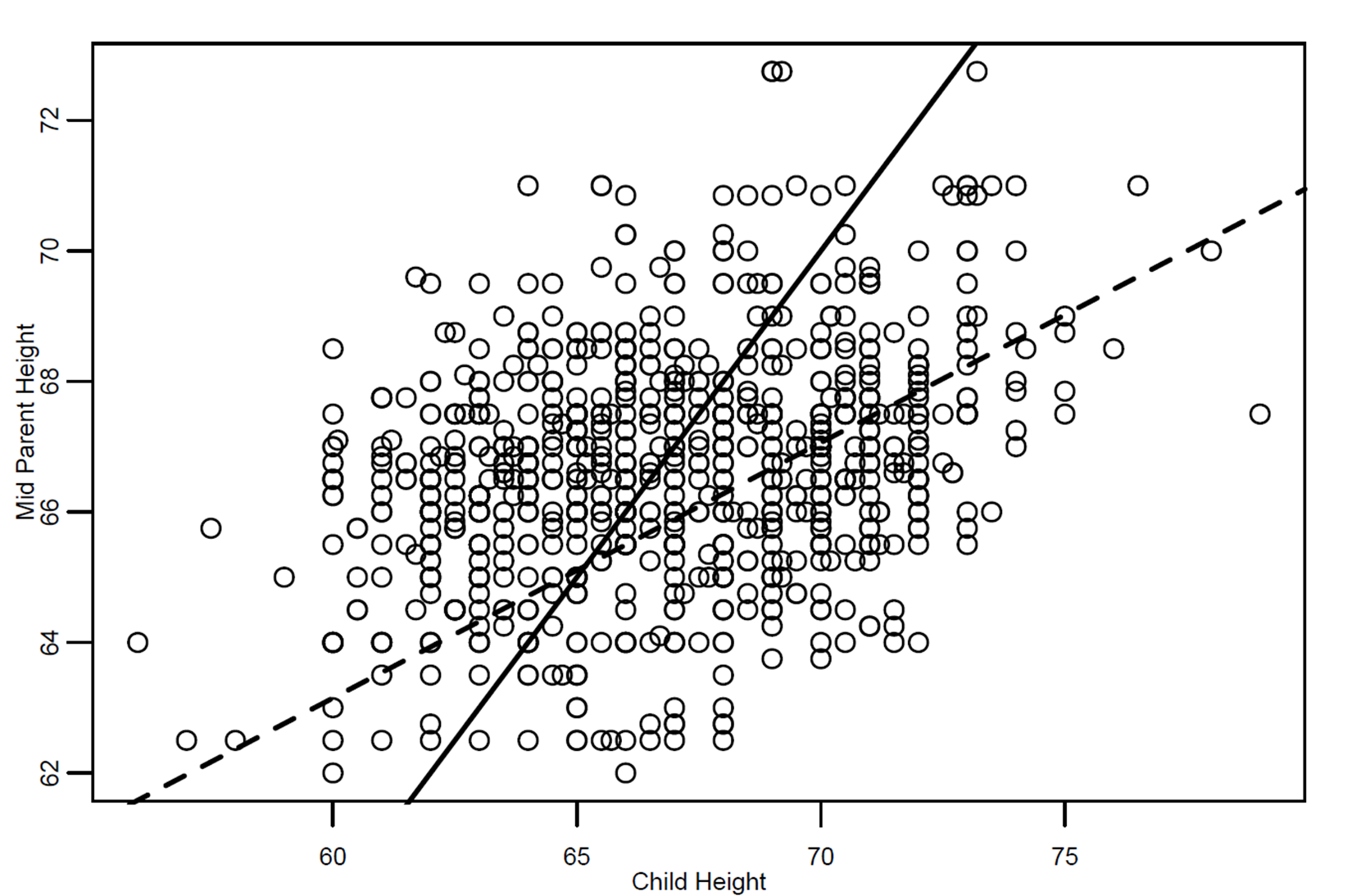
The figure shows a scatter plot of data with two lines. The darker straight line represents the equality line, that is, the average height of the parents is equal to that of the children. The straighter dotted line, on the other hand, represents the linear regression line (defined by Galton) showing a regression in the height of the children relative to that of the parents. In fact, that line has a slope less than that of the continuous line.

Indeed, the children with tall parents are also tall, but on an average they are not as tall as their parents (the regression line is less than the equality line to the right of the figure). On the contrary, children with short parents are also short, but on an average, they are taller than their parents (the regression line is greater than the equality line to the left of the figure). Galton noted that, in both cases, the height of the children approached the average of the group. In Galton's words, this corresponded to the concept of regression towards mediocrity, hence the name of the statistical analysis technique.

The Galton universal regression law was confirmed by Karl Pearson (Galton's pupil), who collected more than a thousand heights of members of family groups. He found that the average height of the children from a group of short parents was greater than the average height of their fathers' group, and that the average height of the children from a group of tall fathers was lower than the average height of their parents' group. That is, the heights of the tall and short children were regressing toward the average height of all people. This is exactly what we have learned from the observation of the previous graph.