

Deep learning has become one of the most popular and recognizable fields of machine learning and computer science. Thanks to an increase in both available data and computational resources, deep learning algorithms have successfully surpassed previous state-of-the-art results in countless tasks. For several domains, including image recognition and playing Go, deep learning has even exceeded the capabilities of mankind.
It is thus not surprising that many reinforcement learning algorithms have started to utilize deep learning to bolster performance. Many of the reinforcement learning algorithms from the beginning of this chapter rely on deep learning. This book, too, will revolve around deep learning algorithms used to tackle reinforcement learning problems.
The following sections will serve as a refresher on some of the most fundamental concepts of deep learning, including neural networks, backpropagation, and convolution. However, if are unfamiliar with these topics, we highly encourage you to seek other sources for a more in-depth introduction.
A neural network is a type of computational architecture that is composed of layers of perceptrons. A perceptron, first conceived in the 1950s by Frank Rosenblatt, models the biological neuron and computes a linear combination of a vector of input. It also outputs a transformation of the linear combination using a non-linear activation, such as the sigmoid function. Suppose a perceptron receives an input vector of

. The output, a, of the perceptron, would be as follows:


Where

are the weights of the perceptron, b is a constant, called the bias, and

is the sigmoid activation function that outputs a value between 0 and 1.
Perceptrons have been widely used as a computational model to make decisions. Suppose the task was to predict the likelihood of sunny weather the next day. Each

would represent a variable, such as the temperature of the current day, humidity, or the weather of the previous day. Then,

would compute a value that reflects how likely it is that there will be sunny weather tomorrow. If the model has a good set of values for

, it is able to make accurate decisions.
In a typical neural network, there are multiple layers of neurons, where each neuron in a given layer is connected to all neurons in the prior and subsequent layers. Hence these layers are also referred to as fully-connected layers. The weights of a given layer, l, can be represented as a matrix, Wl:


Where each wij denotes the weight between the i neuron of the previous layer and the j neuron of this layer. Bl denotes a vector of biases, one for each neuron in the l layer. Hence, the activation, al, of a given layer, l, can be defined as follows:


Where a0(x) is just the input. Such neural networks with multiple layers of neurons are called multilayer perceptrons (MLP). There are three components in an MLP: the input layer, the hidden layers, and the output layer. The data flows from the input layer, transformed through a series of linear and non-linear functions in the hidden layers, and is outputted from the output layer as a decision or a prediction. Hence this architecture is also referred to as a feed-forward network. The following diagram shows what a fully-connected network would look like:
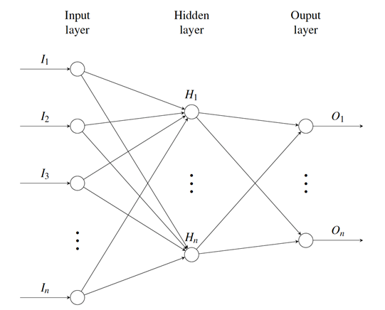
Figure 6: A sketch of a multilayer perceptron
As mentioned previously, a neural network's performance depends on how good the values of W are (for simplicity, we will refer to both the weights and biases as W). When the whole network grows in size, it becomes untenable to manually determine the optimal weights for each neuron in every layer. Therefore, we rely on backpropagation, an algorithm that iteratively and automatically updates the weights of every neuron.
To update the weights, we first need the ground truth, or the target value that the neural network tries to output. To understand what this ground truth could look like, we formulate a sample problem. The MNIST dataset is a large repository of 28x28 images of handwritten digits. It contains 70,000 images in total and serves as a popular benchmark for machine learning models. Given ten different classes of digits (from zero to nine), we would like to identify which digit class a given images belongs to. We can represent the ground truth of each image as a vector of length 10, where the index of the class (starting from 0) is marked as 1 and the rest are 0s. For example, an image, x, with a class label of five would have the ground truth of

, where y is the target function we approximate.
What should the neural network look like? If we take each pixel in the image to be an input, we would have 28x28 neurons in the input layer (every image would be flattened to become a 784-dimensional vector). Moreover, because there are 10 digit classes, we have 10 neurons in the output layer, each neuron producing a sigmoid activation for a given class. There can be an arbitrary number of neurons in the hidden layers.
Let f represent the sequence of transformations that the neural network computes, parameterized by the weights, W. f is essentially an approximation of the target function, y, and maps the 784-dimensional input vector to a 10 dimensional output prediction. We classify the image according to the index of the largest sigmoid output.
Now that we have formulated the ground truth, we can measure the distance between it and the network's prediction. This error is what allows the network to update its weights. We define the error function E(W) as follows:

The goal of backpropagation is to minimize E by finding the right set of W. This minimization is an optimization problem whereby we use gradient descent to iteratively compute the gradients of E with respect to W and propagate them through the network starting from the output layer.
Unfortunately, an in-depth explanation of backpropagation is outside the scope of this introductory chapter. If you are unfamiliar with this concept, we highly encourage you to study it first.
Using backpropagation, we are now able to train large networks automatically. This has led to the development of increasingly complex neural network architectures. One example is the convolutional neural network (CNN). There are mainly three types of layers in a CNN: the convolutional layer, the pooling layer, and the fully-connected layer. The fully-connected layer is identical to the standard neural network discussed previously. In the convolutional layer, weights are part of convolutional kernels. Convolution on a two-dimensional array of image pixels is defined as the following:

Where f(u, v) is the pixel intensity of the input at coordinate (u, v), and g(x-u, y-v) is the weight of the convolutional kernel at that location.
A convolutional layer comprises a stack of convolutional kernels; hence the weights of a convolutional layer can be visualized as a three-dimensional box as opposed to the two-dimensional array that we defined for fully-connected layers. The output of a single convolutional kernel applied to an input is also a two-dimensional mapping, which we call a filter. Because there are multiple kernels, the output of a convolutional layer is again a three-dimensional box, which can be referred to as a volume.
Finally, the pooling layer reduces the size of the input by taking m*m local patches of pixels and outputting a scalar. The max-pooling layer takes m*m patches and outputs the greatest value among the patch of pixels.
Given an input volume of the (32, 32, 3) shape—corresponding to height, width, and depth (channels)—a max-pooling layer with a pooling size of 2x2 will output a volume of the (16, 16, 3) shape. The input to the CNN are usually images, which can also be viewed as volumes where the depth corresponds to RGB channels.
The following is a depiction of a typical convolutional neural network:
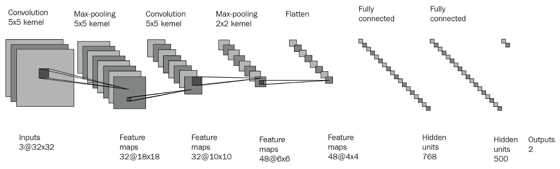
Figure 7: An example convolutional neural network
The main advantage of a CNN over a standard neural network is that the former is able to learn visual and spatial features of the input, while for the latter such information is lost due to flattening input data into a vector. CNNs have made significant strides in the field of computer vision, starting with increased classification accuracies of MNIST data and object recognition, semantic segmentation, and other domains. CNNs have many applications in real life, from facial detection in social media to autonomous vehicles. Recent approaches have also applied CNNs to natural language processing and text classification tasks to produce state-of-the-art results.
Now that we have covered the basics of machine learning, we will go through our first implementation exercise.
In this section, we will implement a simple convolutional neural network in TensorFlow to solve an image classification task. As the rest of this book will be heavily reliant on TensorFlow and CNNs, we highly recommend that you become sufficiently familiar with implementing deep learning algorithms using this framework.
TensorFlow, developed by Google in 2015, is one of the most popular deep learning frameworks in the world. It is used widely for research and commercial projects and boasts a rich set of APIs and functionalities to help researchers and practitioners develop deep learning models. TensorFlow programs can run on GPUs as well as CPUs, and thus abstract the GPU programming to make development more convenient.
Throughout this book, we will be using TensorFlow exclusively, so make sure you are familiar with the basics as you progress through the chapters.
Note
Visit https://www.tensorflow.org/ for a complete set of documentation and other tutorials.
Those who have experience with deep learning have most likely heard about the MNIST dataset. It is one of the most widely-used image datasets, serving as a benchmark for tasks such as image classification and image generation, and is used by many computer vision models:
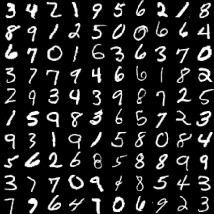
Figure 8: The MNIST dataset (reference at end of chapter)
There are several problems with MNIST, however. First of all, the dataset is too easy, since a simple convolutional neural network is able to achieve 99% test accuracy. In spite of this, the dataset is used far too often in research and benchmarks. The F-MNIST dataset, produced by the online fashion retailer Zalando, is a more complex, much-needed upgrade to MNIST:
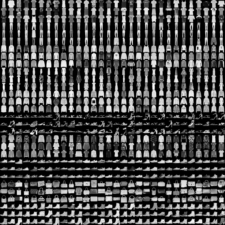
Figure 9: The Fashion-MNIST dataset (taken from https://github.com/zalandoresearch/fashion-mnist, reference at the end of this chapter)
Instead of digits, the F-MNIST dataset includes photos of ten different clothing types (ranging from t-shirts to shoes) compressed in to 28x28 monochrome thumbnails. Hence, F-MNIST serves as a convenient drop-in replacement to MNIST and is increasingly gaining popularity in the community. Hence we will train our CNN on F-MNIST as well. The preceding table maps each label index to its class:
Index | Class |
0 | T-shirt/top |
1 | Trousers |
2 | Pullover |
3 | Dress |
4 | Coat |
5 | Sandal |
6 | Shirt |
7 | Sneaker |
8 | Bag |
9 | Ankle boot |
In the following subsections, we will design a convolutional neural network that will learn to classify data from this dataset.
Multiple deep learning frameworks have already implemented APIs for loading the F-MNIST dataset, including TensorFlow. For our implementation, we will be using Keras, another popular deep learning framework that is integrated with TensorFlow. The Keras datasets module provides a highly convenient interface for loading the datasets as numpy arrays.
Finally, we can start coding! For this exercise, we only need one Python module, which we will call cnn.py. Open up your favorite text editor or IDE, and let's get started.
Our first step is to declare the modules that we are going to use:
import logging
import os
import sys

logger = logging.getLogger(__name__)

import tensorflow as tf
import numpy as np
from keras.datasets import fashion_mnist
from keras.utils import np_utils
The following describes what each module is for and how we will use it:
Module(s) | Purpose |
| For printing statistics as we run the code |
| For interacting with the operating system, including writing files |
| The main TensorFlow library |
| An optimized library for vector calculations and simple data processing |
| For downloading the F-MNIST dataset |
We will implement our CNN as a class called SimpleCNN. The __init__ constructor takes a number of parameters:
class SimpleCNN(object):

def __init__(self, learning_rate, num_epochs, beta, batch_size):
self.learning_rate = learning_rate
self.num_epochs = num_epochs
self.beta = beta
self.batch_size = batch_size
self.save_dir = "saves"
self.logs_dir = "logs"
os.makedirs(self.save_dir, exist_ok=True)
        os.makedirs(self.logs_dir, exist_ok=True)
self.save_path = os.path.join(self.save_dir, "simple_cnn")
self.logs_path = os.path.join(self.logs_dir, "simple_cnn")
The parameters our SimpleCNN is initialized with are described here:
Parameter | Purpose |
| The learning rate for the optimization algorithm |
| The number of epochs it takes to train the network |
| A float value (between 0 and 1) that controls the strength of the L2-penalty |
| The number of images to train on in a single step |
Moreover, save_dir and save_path refer to the locations where we will store our network's parameters. logs_dir and logs_path refer to the locations where the statistics of the training run will be stored (we will show how we can retrieve these logs later).
Now, in this section, we will see two methods that can be used to build the function, which are:
- build method
- fit method
The first method we will define for our SimpleCNN class is the build method, which is responsible for building the architecture of our CNN. Our build method takes two pieces of input: the input tensor and the number of classes it should expect:
def build(self, input_tensor, num_classes):
"""
    Builds a convolutional neural network according to the input shape and the number of classes.
    Architecture is fixed.

    Args:
        input_tensor: Tensor of the input
        num_classes: (int) number of classes

    Returns:
        The output logits before softmax
    """
We will first initializetf.placeholder, called is_training. TensorFlow placeholders are like variables that don't have values. We only pass them values when we actually train the network and call the relevant operations:
with tf.name_scope("input_placeholders"):
self.is_training = tf.placeholder_with_default(True, shape=(), name="is_training")
The tf.name_scope(...) block allows us to name our operations and tensors properly. While this is not absolutely necessary, it helps us organize our code better and will help us to visualize the network. Here, we define a tf.placeholder_with_default called is_training, which has a default value of True. This placeholder will be used for our dropout operations (since dropout has different modes during training and inference).
Note
Naming your operations and tensors is considered a good practice. It helps you organize your code.
Our next step is to define the convolutional layers of our CNN. We make use of three different kinds of layers to create multiple layers of convolutions: tf.layers.conv2d, tf.max_pooling2d, and tf.layers.dropout:
with tf.name_scope("convolutional_layers"):
    conv_1 = tf.layers.conv2d(
input_tensor,
filters=16,
kernel_size=(5, 5),
strides=(1, 1),
padding="SAME",
activation=tf.nn.relu,
kernel_regularizer=tf.contrib.layers.l2_regularizer(scale=self.beta),
name="conv_1")
    conv_2 = tf.layers.conv2d(
        conv_1,
filters=32,
kernel_size=(3, 3),
strides=(1, 1),
padding="SAME",
activation=tf.nn.relu,
kernel_regularizer=tf.contrib.layers.l2_regularizer(scale=self.beta),
name="conv_2")
    pool_3 = tf.layers.max_pooling2d(
        conv_2,
pool_size=(2, 2),
strides=1,
padding="SAME",
name="pool_3"
)
    drop_4 = tf.layers.dropout(pool_3, training=self.is_training, name="drop_4")

    conv_5 = tf.layers.conv2d(
        drop_4,
filters=64,
kernel_size=(3, 3),
strides=(1, 1),
padding="SAME",
activation=tf.nn.relu,
kernel_regularizer=tf.contrib.layers.l2_regularizer(scale=self.beta),
name="conv_5")
    conv_6 = tf.layers.conv2d(
        conv_5,
filters=128,
kernel_size=(3, 3),
strides=(1, 1),
padding="SAME",
activation=tf.nn.relu,
kernel_regularizer=tf.contrib.layers.l2_regularizer(scale=self.beta),
name="conv_6")
    pool_7 = tf.layers.max_pooling2d(
        conv_6,
pool_size=(2, 2),
strides=1,
padding="SAME",
name="pool_7"
)
    drop_8 = tf.layers.dropout(pool_7, training=self.is_training, name="drop_8")
Here are some explanations of the parameters:
Parameter | Type | Description |
|
| Number of filters output by the convolution. |
| Tuple of | The shape of the kernel. |
| Tuple of | The shape of the max-pooling window. |
|
| The number of pixels to slide across per convolution/max-pooling operation. |
|
| Whether to add padding (SAME) or not (VALID). If padding is added, the output shape of the convolution remains the same as the input shape. |
|
| A TensorFlow activation function. |
|
| Which regularization to use for the convolutional kernel. The default value is |
|
| A tensor/placeholder that tells the dropout operation whether the forward pass is for training or for inference. |
In the preceding table, we have specified the convolutional architecture to have the following sequence of layers:
CONV | CONV | POOL | DROPOUT | CONV | CONV | POOL | DROPOUT
However, you are encouraged to explore different configurations and architectures. For example, you could add batch-normalization layers to improve the stability of training.
Finally, we add the fully-connected layers that lead to the output of the network:
with tf.name_scope("fully_connected_layers"):
    flattened = tf.layers.flatten(drop_8, name="flatten")
    fc_9 = tf.layers.dense(
        flattened,
units=1024,
activation=tf.nn.relu,
kernel_regularizer=tf.contrib.layers.l2_regularizer(scale=self.beta),
name="fc_9"
)
    drop_10 = tf.layers.dropout(fc_9, training=self.is_training, name="drop_10")
    logits = tf.layers.dense(
        drop_10,
units=num_classes,
kernel_regularizer=tf.contrib.layers.l2_regularizer(scale=self.beta),
name="logits"
)

return logits
tf.layers.flatten turns the output of the convolutional layers (which is 3-D) into a single vector (1-D) so that we can pass them through the tf.layers.dense layers. After going through two fully-connected layers, we return the final output, which we define as logits.
Notice that in the final tf.layers.dense layer, we do not specify an activation. We will see why when we move on to specifying the training operations of the network.
Next, we implement several helper functions. _create_tf_dataset takes two instances of numpy.ndarray and turns them into TensorFlow tensors, which can be directly fed into a network. _log_loss_and_acc simply logs training statistics, such as loss and accuracy:
def _create_tf_dataset(self, x, y):
    dataset = tf.data.Dataset.zip((
            tf.data.Dataset.from_tensor_slices(x),
            tf.data.Dataset.from_tensor_slices(y)
        )).shuffle(50).repeat().batch(self.batch_size)
return dataset

def _log_loss_and_acc(self, epoch, loss, acc, suffix):
    summary = tf.Summary(value=[
        tf.Summary.Value(tag="loss_{}".format(suffix), simple_value=float(loss)),
        tf.Summary.Value(tag="acc_{}".format(suffix), simple_value=float(acc))
    ])
self.summary_writer.add_summary(summary, epoch)The last method we will implement for our SimpleCNN is the fit method. This function triggers training for our CNN. Our fit method takes four input:
Argument | Description |
| Training data |
| Training labels |
| Test data |
| Test labels |
The first step of fit is to initializetf.Graph andtf.Session. Both of these objects are essential to any TensorFlow program.tf.Graph represents the graph in which all the operations for our CNN are defined. You can think of it as a sandbox where we define all the layers and functions.tf.Session is the class that actually executes the operations defined intf.Graph:
def fit(self, X_train, y_train, X_valid, y_valid):
"""
    Trains a CNN on given data

    Args:
        numpy.ndarrays representing data and labels respectively
    """
graph = tf.Graph()
with graph.as_default():
        sess = tf.Session()
We then create datasets using TensorFlow's Dataset API and the _create_tf_dataset method we defined earlier:
train_dataset = self._create_tf_dataset(X_train, y_train)
valid_dataset = self._create_tf_dataset(X_valid, y_valid)

# Creating a generic iterator
iterator = tf.data.Iterator.from_structure(train_dataset.output_types,
                                           train_dataset.output_shapes)
next_tensor_batch = iterator.get_next()

# Separate training and validation set init ops
train_init_ops = iterator.make_initializer(train_dataset)
valid_init_ops = iterator.make_initializer(valid_dataset)

input_tensor, labels = next_tensor_batch
tf.data.Iterator builds an iterator object that outputs a batch of images every time we call iterator.get_next(). We initialize a dataset each for the training and testing data. The result of iterator.get_next() is a tuple of input images and corresponding labels.
The former is input_tensor, which we feed into the build method. The latter is used for calculating the loss function and backpropagation:
num_classes = y_train.shape[1]

# Building the network
logits = self.build(input_tensor=input_tensor, num_classes=num_classes)
logger.info('Built network')

prediction = tf.nn.softmax(logits, name="predictions")
loss_ops = tf.reduce_mean(tf.nn.softmax_cross_entropy_with_logits_v2(
labels=labels, logits=logits), name="loss")
logits (the non-activated outputs of the network) are fed into two other operations: prediction, which is just the softmax over logits to obtain normalized probabilities over the classes, and loss_ops, which calculates the mean categorical cross-entropy between the predictions and the labels.
We then define the backpropagation algorithm used to train the network and the operations used for calculating accuracy:
optimizer = tf.train.AdamOptimizer(learning_rate=self.learning_rate)
train_ops = optimizer.minimize(loss_ops)

correct = tf.equal(tf.argmax(prediction, 1), tf.argmax(labels, 1), name="correct")
accuracy_ops = tf.reduce_mean(tf.cast(correct, tf.float32), name="accuracy")
We are now done building the network along with its optimization algorithms. We use tf.global_variables_initializer() to initialize the weights and operations of our network. We also initialize the tf.train.Saver and tf.summary.FileWriter objects. The tf.train.Saver object saves the weights and architecture of the network, whereas the latter keeps track of various training statistics:
initializer = tf.global_variables_initializer()

logger.info('Initializing all variables')
sess.run(initializer)
logger.info('Initialized all variables')

sess.run(train_init_ops)
logger.info('Initialized dataset iterator')
self.saver = tf.train.Saver()
self.summary_writer = tf.summary.FileWriter(self.logs_path)
Finally, once we have set up everything we need, we can implement the actual training loop. For every epoch, we keep track of the training cross-entropy loss and accuracy of the network. At the end of every epoch, we save the updated weights to disk. We also calculate the validation loss and accuracy every 10 epochs. This is done by calling sess.run(...), where the arguments to this function are the operations that the sess object should execute:
logger.info("Training CNN for {} epochs".format(self.num_epochs))
for epoch_idx in range(1, self.num_epochs+1):
    loss, _, accuracy = sess.run([
        loss_ops, train_ops, accuracy_ops
    ])
self._log_loss_and_acc(epoch_idx, loss, accuracy, "train")

if epoch_idx % 10 == 0:
        sess.run(valid_init_ops)
        valid_loss, valid_accuracy = sess.run([
            loss_ops, accuracy_ops
        ], feed_dict={self.is_training: False})
        logger.info("=====================> Epoch {}".format(epoch_idx))
        logger.info("\tTraining accuracy: {:.3f}".format(accuracy))
        logger.info("\tTraining loss: {:.6f}".format(loss))
        logger.info("\tValidation accuracy: {:.3f}".format(valid_accuracy))
        logger.info("\tValidation loss: {:.6f}".format(valid_loss))
self._log_loss_and_acc(epoch_idx, valid_loss, valid_accuracy, "valid")

# Creating a checkpoint at every epoch
self.saver.save(sess, self.save_path)
And that completes our fit function. Our final step is to create the script for instantiating the datasets, the neural network, and then running training, which we will write at the bottom of cnn.py.
We will first configure our logger and load the dataset using the Keras fashion_mnist module, which loads the training and testing data:
if __name__ == "__main__":
    logging.basicConfig(stream=sys.stdout,
level=logging.DEBUG,
format='%(asctime)s %(name)-12s %(levelname)-8s %(message)s')
    logger = logging.getLogger(__name__)

    logger.info("Loading Fashion MNIST data")
    (X_train, y_train), (X_test, y_test) = fashion_mnist.load_data()
We then apply some simple preprocessing to the data. The Keras API returns numpy arrays of the (Number of images, 28, 28) shape.
However, what we actually want is (Number of images, 28, 28, 1), where the third axis is the channel axis. This is required because our convolutional layers expect input that have three axes. Moreover, the pixel values themselves are in the range of [0, 255]. We will divide them by 255 to get a range of [0, 1]. This is a common technique that helps stabilize training.
Furthermore, we turn the labels, which are simply an array of label indices, into one-hot encodings:
logger.info('Shape of training data:')
logger.info('Train: {}'.format(X_train.shape))
logger.info('Test: {}'.format(X_test.shape))

logger.info('Adding channel axis to the data')
X_train = X_train[:,:,:,np.newaxis]
X_test = X_test[:,:,:,np.newaxis]

logger.info("Simple transformation by dividing pixels by 255")
X_train = X_train / 255.
X_test = X_test / 255.

X_train = X_train.astype(np.float32)
X_test = X_test.astype(np.float32)
y_train = y_train.astype(np.float32)
y_test = y_test.astype(np.float32)
num_classes = len(np.unique(y_train))

logger.info("Turning ys into one-hot encodings")
y_train = np_utils.to_categorical(y_train, num_classes=num_classes)
y_test = np_utils.to_categorical(y_test, num_classes=num_classes)
We then define the input to the constructor of our SimpleCNN. Feel free to tweak the numbers to see how they affect the performance of the model:
cnn_params = {
"learning_rate": 3e-4,
"num_epochs": 100,
"beta": 1e-3,
"batch_size": 32
}
And finally, we instantiate SimpleCNN and call its fit method:
logger.info('Initializing CNN')
simple_cnn = SimpleCNN(**cnn_params)
logger.info('Training CNN')
simple_cnn.fit(X_train=X_train,
X_valid=X_test,
y_train=y_train,
y_valid=y_test)
To run the entire script, all you need to do is run the module:
$ python cnn.pyAnd that's it! You have successfully implemented a convolutional neural network in TensorFlow to train on the F-MNIST dataset. To track the progress of the training, you can simply look at the output in your terminal/editor. You should see an output that resembles the following:
$ python cnn.py
Using TensorFlow backend.
2018-07-29 21:21:55,423 __main__ INFO Loading Fashion MNIST data
2018-07-29 21:21:55,686 __main__ INFO Shape of training data:
2018-07-29 21:21:55,687 __main__ INFO Train: (60000, 28, 28)
2018-07-29 21:21:55,687 __main__ INFO Test: (10000, 28, 28)
2018-07-29 21:21:55,687 __main__ INFO Adding channel axis to the data
2018-07-29 21:21:55,687 __main__ INFO Simple transformation by dividing pixels by 255
2018-07-29 21:21:55,914 __main__ INFO Turning ys into one-hot encodings
2018-07-29 21:21:55,914 __main__ INFO Initializing CNN
2018-07-29 21:21:55,914 __main__ INFO Training CNN
2018-07-29 21:21:58,365 __main__ INFO Built network
2018-07-29 21:21:58,562 __main__ INFO Initializing all variables
2018-07-29 21:21:59,284 __main__ INFO Initialized all variables
2018-07-29 21:21:59,639 __main__ INFO Initialized dataset iterator
2018-07-29 21:22:00,880 __main__ INFO Training CNN for 100 epochs
2018-07-29 21:24:23,781 __main__ INFO =====================> Epoch 10
2018-07-29 21:24:23,781 __main__ INFO Training accuracy: 0.406
2018-07-29 21:24:23,781 __main__ INFO Training loss: 1.972021
2018-07-29 21:24:23,781 __main__ INFO Validation accuracy: 0.500
2018-07-29 21:24:23,782 __main__ INFO Validation loss: 2.108872
2018-07-29 21:27:09,541 __main__ INFO =====================> Epoch 20
2018-07-29 21:27:09,541 __main__ INFO Training accuracy: 0.469
2018-07-29 21:27:09,541 __main__ INFO Training loss: 1.573592
2018-07-29 21:27:09,542 __main__ INFO Validation accuracy: 0.500
2018-07-29 21:27:09,542 __main__ INFO Validation loss: 1.482948
2018-07-29 21:29:57,750 __main__ INFO =====================> Epoch 30
2018-07-29 21:29:57,750 __main__ INFO Training accuracy: 0.531
2018-07-29 21:29:57,750 __main__ INFO Training loss: 1.119335
2018-07-29 21:29:57,750 __main__ INFO Validation accuracy: 0.625
2018-07-29 21:29:57,750 __main__ INFO Validation loss: 0.905031
2018-07-29 21:32:45,921 __main__ INFO =====================> Epoch 40
2018-07-29 21:32:45,922 __main__ INFO Training accuracy: 0.656
2018-07-29 21:32:45,922 __main__ INFO Training loss: 0.896715
2018-07-29 21:32:45,922 __main__ INFO Validation accuracy: 0.719
2018-07-29 21:32:45,922 __main__ INFO Validation loss: 0.847015
Another thing to check out is TensorBoard, a visualization tool developed by the developers of TensorFlow, to graph the model's accuracy and loss. The tf.summary.FileWriter object we have used serves this purpose. You can run TensorBoard with the following command:
$ tensorboard --logdir=logs/logs is where our SimpleCNN model writes the statistics to. TensorBoard is a great tool for visualizing the structure of our tf.Graph, as well as seeing how statistics such as accuracy and loss change over time. By default, the TensorBoard logs can be accessed by pointing your browser to localhost:6006:
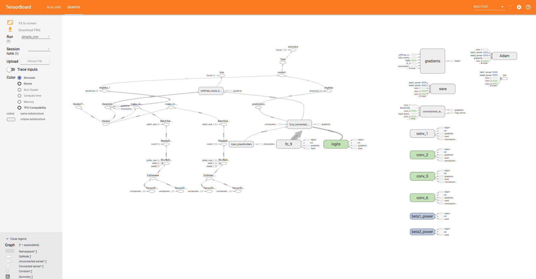
Figure 10: TensorBoard and its visualization of our CNN
Congratulations! We have successfully implemented a convolutional neural network using TensorFlow. However, the CNN we implemented is rather rudimentary, and only achieves mediocre accuracy—the challenge to the reader is to tweak the architecture to improve its performance.