-
Book Overview & Buying
-
Table Of Contents

Hands-On Image Processing with Python
By :
Hands-On Image Processing with Python
By:
Overview of this book
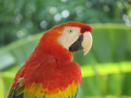
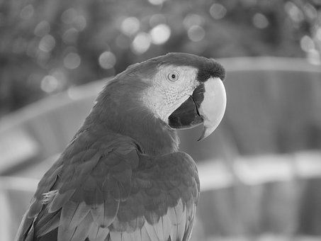
Image processing plays an important role in our daily lives with various applications such as in social media (face detection), medical imaging (X-ray, CT-scan), security (fingerprint recognition) to robotics & space. This book will touch the core of image processing, from concepts to code using Python.
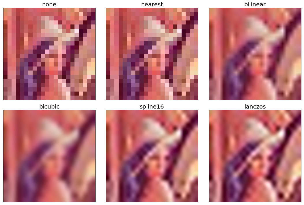
The book will start from the classical image processing techniques and explore the evolution of image processing algorithms up to the recent advances in image processing or computer vision with deep learning. We will learn how to use image processing libraries such as PIL, scikit-mage, and scipy ndimage in Python. This book will enable us to write code snippets in Python 3 and quickly implement complex image processing algorithms such as image enhancement, filtering, segmentation, object detection, and classification. We will be able to use machine learning models using the scikit-learn library and later explore deep CNN, such as VGG-19 with Keras, and we will also use an end-to-end deep learning model called YOLO for object detection. We will also cover a few advanced problems, such as image inpainting, gradient blending, variational denoising, seam carving, quilting, and morphing.
By the end of this book, we will have learned to implement various algorithms for efficient image processing.
Table of Contents (20 chapters)
Title Page

Copyright and Credits
Dedication
About Packt
Contributors
Preface
 Free Chapter
Getting Started with Image Processing
Sampling, Fourier Transform, and Convolution
Convolution and Frequency Domain Filtering
Image Enhancement
Image Enhancement Using Derivatives
Morphological Image Processing
Extracting Image Features and Descriptors
Image Segmentation
Classical Machine Learning Methods in Image Processing
Deep Learning in Image Processing - Image Classification
Deep Learning in Image Processing - Object Detection, and more
Additional Problems in Image Processing
Other Books You May Enjoy
Index