In this section, we will take a look at how to detect breast cancer with a support vector machine (SVM). We're also going to throw in a k-nearest neighbors (KNN) clustering algorithm, and compare the results. We will be using the conda distribution, which is a great way to download and install Python since conda is a package manager, meaning that it makes downloading and installing the necessary packages easy and straightforward. With conda, we're also going to install the Jupyter Notebook, which we will use to program in Python. This will make sharing code and collaborating across different platforms much easier.

Now, let's go through the steps required to use Anaconda, as follows:

1. Start by downloading conda, and make sure that is in your Path variables.
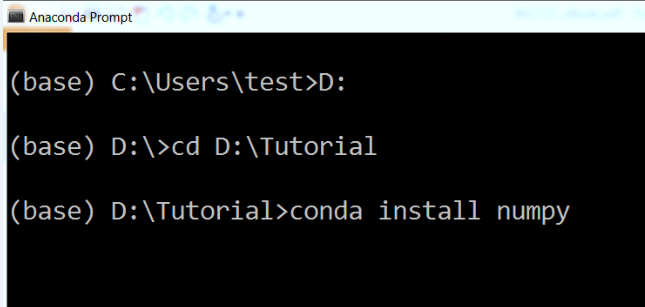
2. Open up a Command Prompt, which is the best way to use conda, and go into the Tutorial folder.
3. If conda is in your Path variables, you can simply type conda install, followed by whichever package you need. We're going to be using numpy, so we will type that, as you can see in the following screenshot:

4. To start the Jupyter Notebook, simply type jupyter notebook and press Enter. If conda is in the path, Jupyter will be found, as well, because it's located in the same folder. It will start to load up, as shown in the following screenshot:

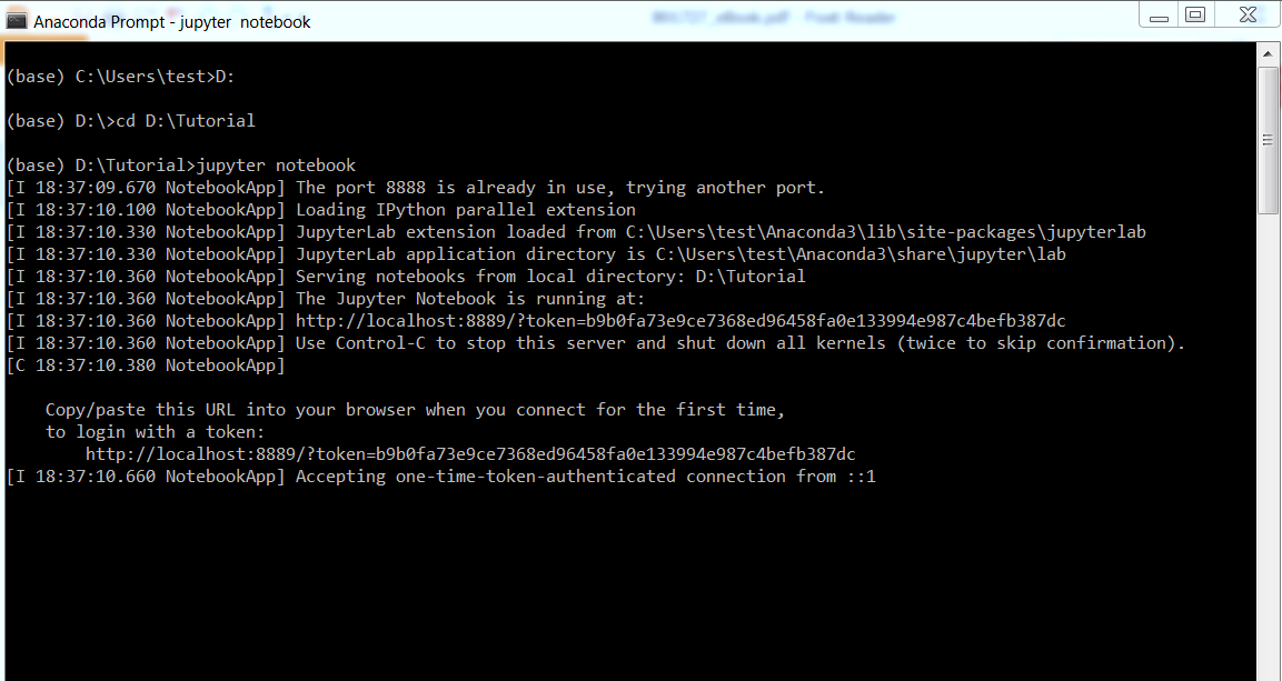
The folder that we're in when we type jupyter notebook is where it will open up on the web browser.

5. After that, click on New, and select Python [default]. Using Python 2.7 would be preferable, as it seems to be more of a standard in the industry.
6. To check that we all have the same versions, we will conduct an import step.
7. Rename the notebook to Breast Cancer Detection with Machine Learning.
8. Import sys, so that we can check whether we're using Python 2.7.

9. We will import numpy, matplotlib, pandas, and the sklearn packages and print their versions. We can view the changes in the following screenshot:

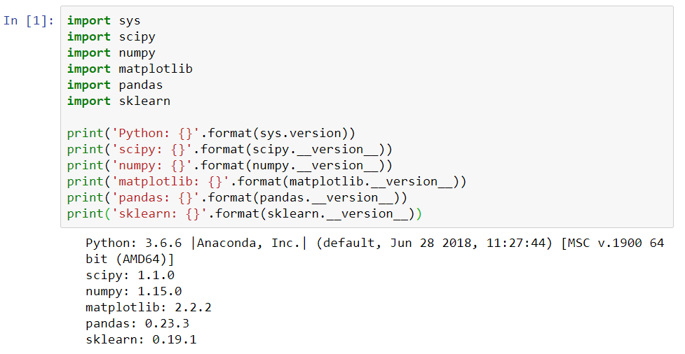
To run the cell in Jupyter Notebook, simply press Shift + Enter. A number will pop up when it completes, and it'll print out the statements. Once again, if we encounter errors in this step and we are unable to import any of the preceding packages, we have to exit the Jupyter Notebook, type conda install, and mention whichever package we are missing in the Terminal. These will then be installed. The necessary packages and versions are shown as follows:

• Python 2.7
• 1.14 for NumPy
• Matplotlib
• Pandas
• Sklearn

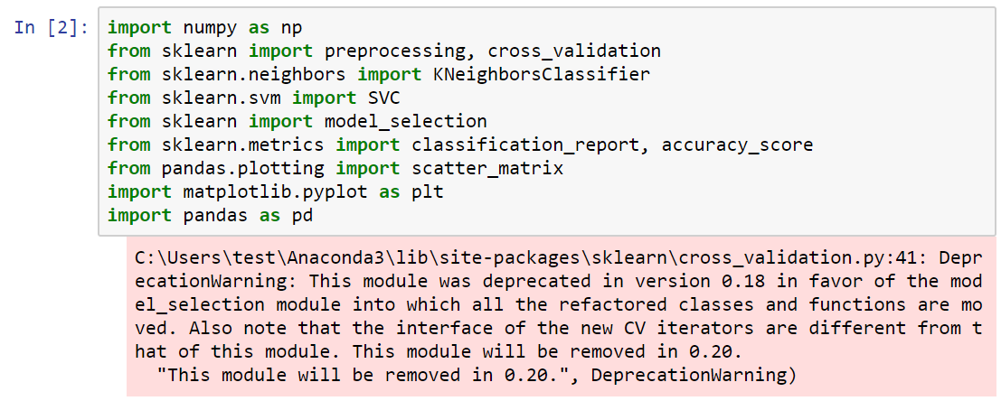
The following screenshot illustrates how to import these libraries in the specific way that we're going to use them in this project:

In the following steps, we will look at how to import the different arguments in these libraries:

1. First, we will import NumPy, using the command import numpy as np.
2. Next, we will import the various classes and functions in sklearn - namely, preprocessing and cross_validation.
3. From neighbors, we will import KNeighborsClassifier, which will be KNN.
4. From sklearn.svm, we will import the support vector classifier (SVC).
5. We're going to do model_selection, so that we can use both KNN and SVC in one step.
6. We will then get some metrics, in which we will import the classification_report, as well as the accuracy_score.
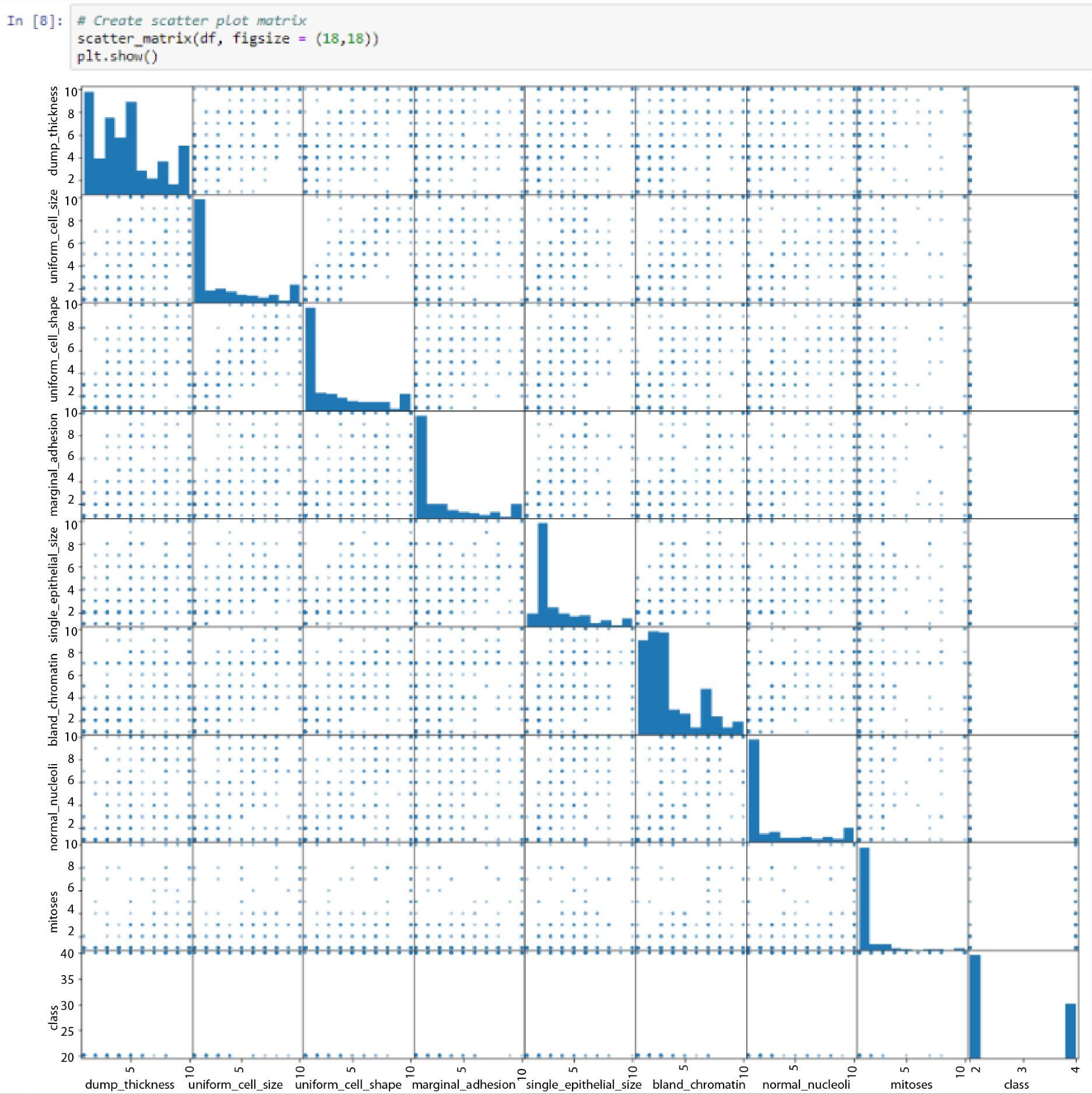
7. From pandas, we need to import plotting, which is the scatter_matrix. This will be useful when we're exploring some data visualizations, before diving into the actual machine learning.
8. Finally, from matplotlib.pyplot, we will import pandas as pd.
9. Now, press Shift + Enter, and make sure that all of the arguments import.

10. Now that we have all of our packages set up, we can move on to loading the dataset. This is where we're going to be getting our information from. We're going to be using the UCI repository, since they have a large collection of datasets for machine learning, and they're free and available for everybody to use.
11. The URL that we're going to use can be imported directly, if we type the whole URL. This is going to import our dataset with 11 different columns. We can see the URL and the various columns in the following screenshot:

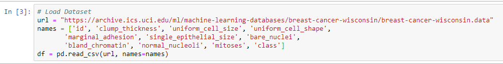
We will then import the cell data. This will include the following aspects:

• The first column will simply be the ID of the cell
• In the second column, we will have clump_thickness
• In the third column, we will have uniform_cell_size
• In the fourth column, we will have uniform_cell_shape
• In the fifth column, we will have marginal_adhesion
• In the sixth column, we will have signle_epithelial_size
• In the seventh column, we will have bare_nuclei
• In the eighth column, we will have bland_chromatin
• In the ninth column, we will have normal_nucleoli
• In the tenth column, we will have mitoses
• And finally, in the eleventh column, we will have class

These are factors that a pathologist would consider to determine whether or not a cell had cancer. When we discuss machine learning in healthcare, it has to be a collaborative project between doctors and computer scientists. While a doctor can help by indicating which factors are important to include, a computer scientist can help by carrying out machine learning. Now, let's move on to the next steps:

1. Since we've got the names of our columns, we will now start a DataFrame.
2. The next step will be to add pd, which stands for pandas. We're going to use the function read_csv_url, which means that the names will be equal to those listed previously.

3. Press Shift + Enter, and make sure that all of the imports are right.
4. We will then have to preprocess our data and carry out some visualizations, as we want to explore the dataset before we begin.

In machine learning, it's very important to understand the data that you're going to be using. This will help you pick which algorithm to use, and understand which results you're actually looking for. It is important to understand, for example, what is considered a good result, because accuracy is not always the most important classification metric. Take a look at the following steps:

1. First, our dataset contains some missing data. To deal with this, we will add a df.replace method.
2. If df.replace gives us a question mark, it means that there's no data there. We're simply going to input the value -99999 and tell Python to ignore that data.
3. We will then perform the print(df.axes) operation, so that we can see the columns. We can see that we have 699 different data points, and each of those cases has 11 different columns.
4. Next, we will print the shape of the dataset using the print(df.shape) operation.

Let's view the output of the preceding steps in the following screenshot:

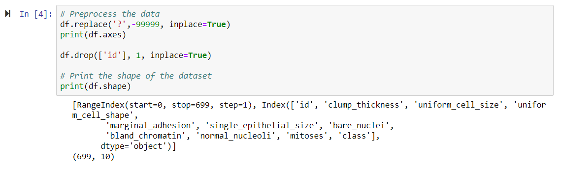
As we now have all of the columns, we can detect whether the tumor is benign (which means it is non-cancerous) or malignant (which means it is cancerous). We now have 10 columns, as we have dropped the ID column.

In the following screenshot, we can see the first cell in our dataset, as well as its different features:

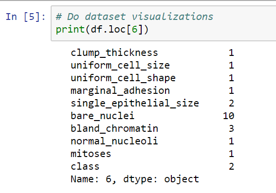
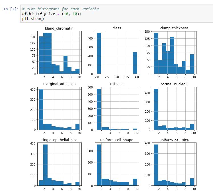
Now let's visualize the parameters of the dataset, in the following steps:

1. We will print the first point, so that we can see what it entails.
2. We have a value of between 0 and 10 in all of the different columns. In the class column, the number 2 represents a benign tumor, and the number 4 represents a malignant tumor. There are 699 cells in the datasets.
3. The next step will be to do a print.describe operation, which gives us the mean, standard deviation, and other aspects for each of our different parameters or features. This is shown in the following screenshot:

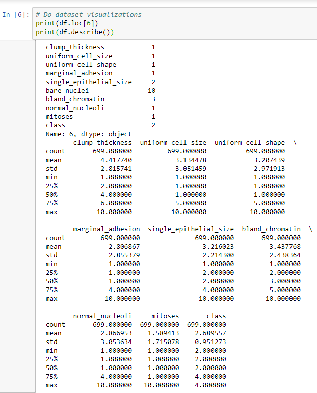
Here, we have a max value of 10 for all of the different columns, apart from the class column, which will either be 2 or 4. The mean is a little closer to 2, so we have a few more benign cases than we do malignant cases. Because the min and the max values are between 1 and 10 for all columns, it means that we've successfully ignored the missing data, so we're not factoring that in. Each column has a relatively low mean, but most of them have a max of 10, which means that we have a case where we hit 10 in all but one of the classes.

Let's get started with data visualization. We will plot histograms for each variable. The steps in the preceding section are important, because we need to understand these datasets if we want to accurately and effectively use machine learning. Otherwise, we're shooting in the dark, and we might spend time on a method that doesn't need to be investigated. We will use the plt method and make a plot, in which we will add the histograms of our dataset and edit the figure sizes, to make them easier to see.

We can see the output in the following screenshot:

As you can see, most of the preceding histograms have the majority of their data at around 1, with some data at a slightly higher value. Each histogram, apart from class, has at least one case where the value is 10. The histogram for clump thickness is pretty evenly distributed, while the histogram for chromatin is skewed to the left.

We will now look at a scatterplot matrix, to see the relationships between some of these variables. A scatterplot matrix is a very useful function to use, because it can tell us whether a linear classifier will be a good classifier for our data, or whether we have to investigate more complicated methods.

We will add a scatter_matrix method and adjust the size to figsize(18, 18), to make it easier to see.

The output, as shown in the following screenshot, indicates the relationship between each variable and every other variable:

All of the variables are listed on both the x and the y axes. Where they intersect, we can see the histograms that we saw previously.

In the block indicated by the mouse cursor in the preceding screenshot, we can see that there is a pretty strong linear relationship between uniform_cell_shape and uniform_cell_size. This is expected. When we go through the preceding screenshot, we can see that some other cells have a good linear relationship. If we look at our classifications, however, there's no easy way to classify these relationships.

In class in the preceding screenshot, we can see that 4 is a malignant classification. We can also see that there are cells that are scored from 1 to 10 on clump_thickness, and were still classified as malignant.

Thus, we come to the conclusion that there aren't any strong relationships between any of the variables of our dataset.

Since we've explored our dataset, let's take a look at how machine learning algorithms can help us to define whether a person has cancer.

The following steps will help you to better understand the machine learning algorithm:

1. The first step that we need to perform is to split our dataset into X and Y datasets for training. We won't train all of the available data, as we need to save some for our validation step. This will help us to determine how well these algorithms can generalize to new data, and not just how well they know the training data.
2. Our X data will contain all of the variables, except for the class column, and our Y data is going to be the class column, which is the classification of whether a tumor is malignant or benign.
3. Next, we will use the train_test_split function, and we will then split our data into y_train, y_test, X_train, and X_test, respectively.

4. In the same line, we will add cross_validation.train_test_split and X, y, test_size. About 20% of our data is fairly standard, so we will make the test size 0.2 to test the data as shown in the following screenshot:

5. Next, we will add a seed, which makes the data reproducible. We will start with a random seed, which will change the results a little bit every time.

6. In scoring, we will add accuracy. This is shown in the following screenshot:

In the preceding section, you learned about how machine learning algorithms can be used for healthcare purposes. We also looked at the testing parameters that are used for this application.