We have just installed and configured our Keras environment, and we can now focus on the implementation of our model based on deep neural networks. When developing a deep learning application, we follow a general pipeline characterized by the following steps:

1. Collecting the data: Everything starts from the data, no doubt about it, but one might wonder where so much data comes from. In practice, it is collected through lengthy procedures that may, for example, derive from measurement campaigns or face-to-face interviews. In all cases, the data is collected in a database so that it can then be analyzed to derive knowledge.

2. Preparing the data: We have collected the data; now we have to prepare it for the next step. Once we have this data, we must make sure it is in a format usable by the algorithm we want to use. To do this, you may need to do some formatting. Recall that some algorithms need data in an integer format, whereas others require data in the form of strings. Finally, others need to be in a special format. We will get to this later, but the specific formatting is usually simple compared to data collection.

The following diagram shows the deep learning process workflow:

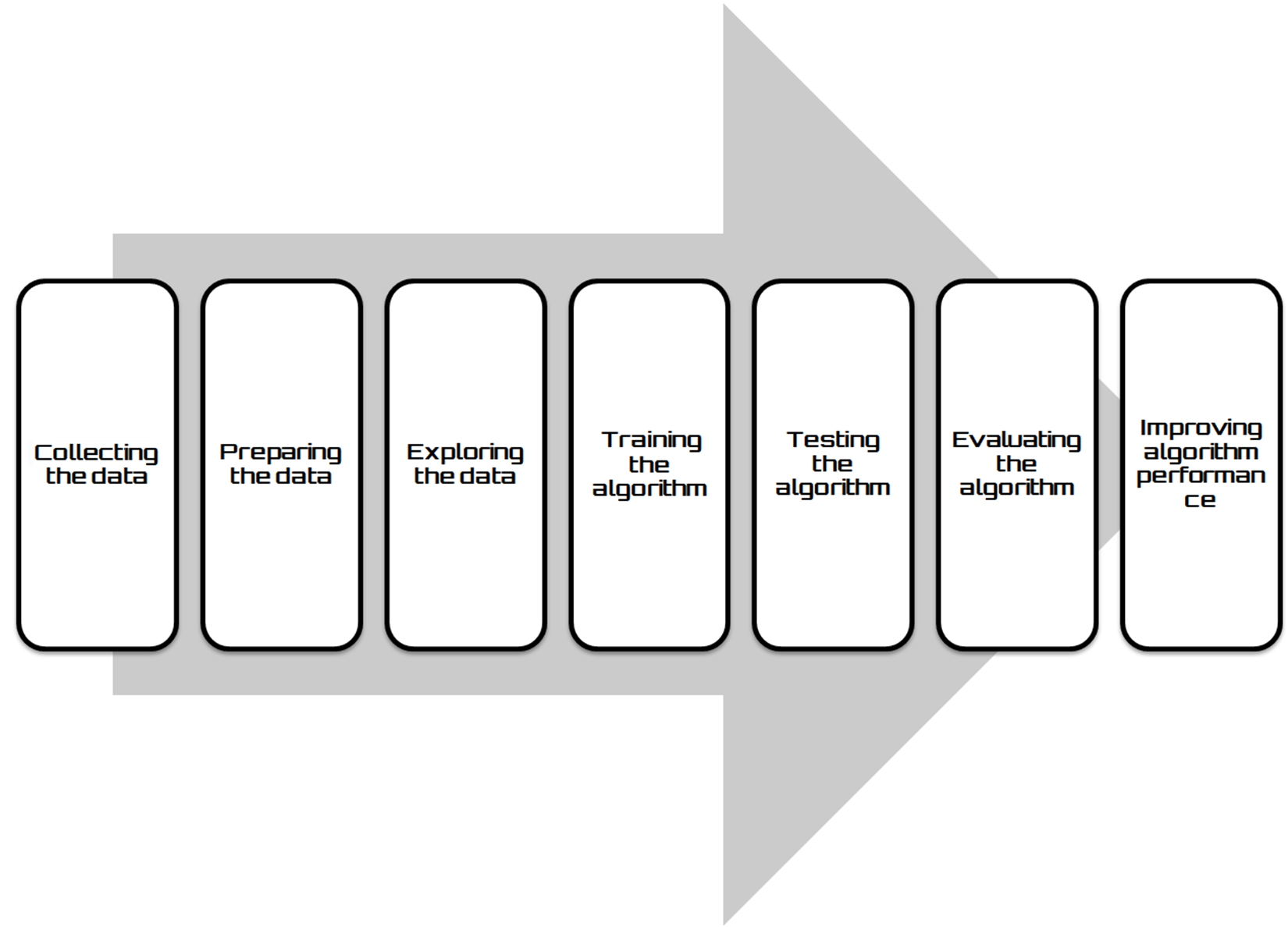
3. Exploring the data: At this point, we can look at data to verify that it is actually working and we do not have a bunch of empty values. In this step, through the use of plots, we can recognize patterns or whether there are some data points that are vastly different from the rest of the set. Plotting data in one, two, or three dimensions can also help.
4. Training the algorithm: Now, let's get serious. In this step, the deep learning begins to work with the definition of the model and the next training round. The model starts to extract knowledge from large amounts of data that we had available. For unsupervised learning, there's no training step because you don't have a target value.
5. Testing the algorithm: In this step, we use the information learned in the previous step to see if the model actually works. The evaluation of an algorithm verifies how well the model approximates the real system. In the case of supervised learning, we have some known values that we can use to evaluate the algorithm. In unsupervised learning, we may need to use some other metrics to evaluate success. In both cases, if we are not satisfied, we can return to the previous steps, change some things, and retry the test.

6. Evaluating the algorithm: We have reached the point where we can apply what has been done so far. We can assess the approximation ability of the model by applying it to real data. The model, preventively trained and tested, is then valued in this phase.
7. Improving algorithm performance: Finally, we can focus on the finishing steps. We've verified that the model works, we have evaluated the performance, and now we are ready to analyze the whole process to identify any possible room for improvement.

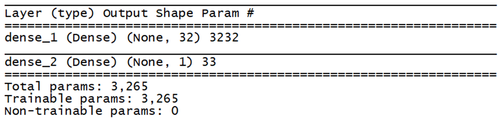
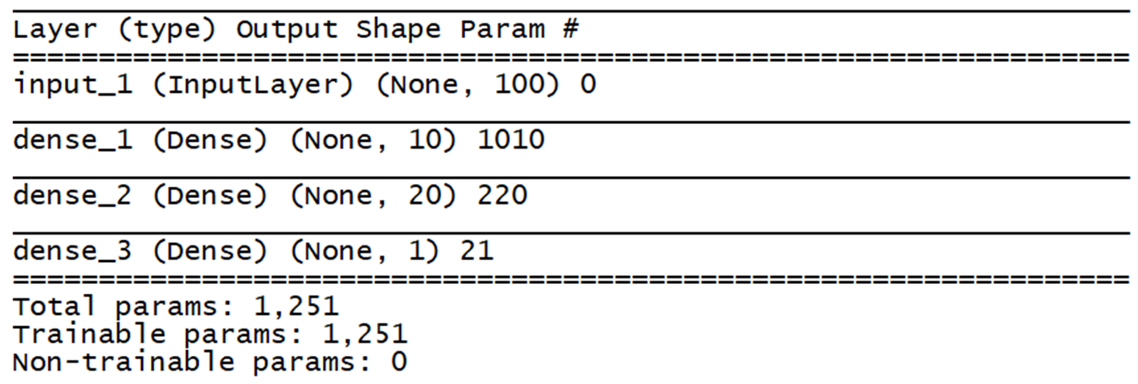
In Keras, there are two ways to define a model—sequential, and functional API. The sequential model lets you create layer-by-layer models for most problems. Limits are dictated by the inability to create models that share levels or that have multiple inputs or outputs. Alternatively, the functional API allows you to create models with greater flexibility. We can easily define models in which the levels are connected in different ways and not just from the previous level to the next. In fact, we can link a layer to any other level, thus creating complex networks.

Keras is structured according to the object-oriented programming methodology. Therefore, the creation of a model is very simple: select the basic architecture and then add the layers necessary to create the desired model. As just mentioned, the sequential model lets you create a layer-by-layer model as a linear stack of layers. However, it is not possible to create models that share levels or that have multiple inputs or outputs.

A sequential model is created by passing a list of layer instances to the constructor. To create a model, we should follow these steps:

1. Import the sequential class from keras.models

2. Stack layers using the .add() method

3. Configure the learning process using the compile() method

4. Import the data

5. Train the model on the train dataset using the .fit() method

The first step is solved by importing the classes that we will use later for the construction of the model. An example of an import is shown in the following command:

from keras.models import Sequential
from keras.layers import Dense, Activation

Three layer classes have been imported: Sequential, Dense, and Activation. Then, we instantiate an object from the Keras.model.Sequential class:

model = Sequential()

All information about your network, such as weights, layers, and operations will be stored in this object.

After instantiating our object, we will move on to adding layers using the add() method:

model.add(Dense(32, activation='relu', input_dim=100))
model.add(Dense(1, activation='sigmoid'))

We have added two Dense layers, which is the basic feedforward fully connected layer.

All operations of a layer can be passed as arguments to the Dense object, as follows:

• Number of hidden units
• Activation function
• Bias
• Weight/bias initialization
• Weight/bias regularization
• Activation regularization

You can create any level in the network using the following command:

model.add (layer_name)

This method will preserve the order of the levels you add. There are lots of layers implemented in Keras. When you add a layer to your model, a gradient operation will be created in the background and it will take care of computing the backward gradient automatically. Before training a model, you need to configure the learning process, which is done via the compile() method; we can see it in the following code block:

model.compile(optimizer='rmsprop',
              loss='binary_crossentropy',
              metrics=['accuracy'])

The three arguments that are passed are as follows:

• An optimizer
• A loss function
• A list of metrics

At this point, we have set the model architecture and before proceeding to the training we have to import the data.

In this case, we generate simple dummy data by performing a random sampling using numpy:

import numpy as np
data = np.random.random((1000, 100))
labels = np.random.randint(2, size=(1000, 1))

To train a model, the fit () method is used, as seen in the following code block:

model.fit(data, labels, epochs=10, batch_size=32)

In this way, we have trained the model, iterating on the data in groups of 32 samples. With these few lines of code, we have already built our first network in Keras. This is a simple example of binary classification that uses a single entry model with two classes.

In Keras, to summarize a model, it is possible to use the summary() function. The summary is returned in text format and includes the following information:

• The layers and their order in the model
• The output shape of each layer
• The number of parameters (weights) in each layer
• The total number of parameters (weights) in the model

To print a summary of the model, we simply type the following command:

model.summary()

In the following screenshot, the results are shown:

Here, we can clearly see the output shape and number of weights in each layer.

The functional API is much better when you want to do something that diverges from the basic idea of having an input, a succession of levels, and an output, for example, models with multiple inputs, multiple outputs, or a more complex internal structure, such as using the output of a given layer as an input to multiple layers or, on the contrary, combining the output of different layers to use them together as an input of another level.

In fact, as already said, the functional API allows you to create models with greater flexibility. We can easily define models in which the levels are connected in different ways and not just from the previous level to the next. In fact, we can link a layer to any other level, thus creating complex networks.

To understand the difference between the two models that Keras offers, we will use a simple example. This is a densely connected network of the type already seen in The Keras sequential model architecture section. In a densely connected network, every input is connected to every output by a weight, which is generally followed by a non-linear activation function. Again, we recommend it for its simplicity. The first step is solved by importing the classes that we will use later for the construction of the model. We will run the example using the following steps:

We will begin by importing the required libraries using the following code block:

from keras.layers import Input, Dense
from keras.models import Model

Three layer classes have been imported: Input, Dense, and Model.

Then, we have to instantiate a Keras Tensor. In fact, in this case we must define an autonomous input level that specifies the shape of the input data (tensor). The input layer accepts a shape argument, which is a tuple indicating the dimensionality of the input data:

InputTensor = Input(shape=(100,))

This returns a tensor.

Now, we can define the layers using the following code block:

H1 = Dense(10, activation='relu')(InputTensor)

The first dense layer is created, which connects the input layer output (InputTensor) as the input to the dense layer, (x). It is this way of connecting layers (layers by layer) that gives the functional API its flexibility. A layer instance is callable on a tensor, and returns a tensor.

Let's move on to the next layer:

H2 = Dense(20, activation='relu')(H1)

So, a second dense layer is created, that connects the Dense layer output, (x), as the input to the other dense layer, (H2).

Let's move on to the final layer creation:

Output = Dense(1, activation='softmax')(H2)

Finally, a third dense layer is created that connects the Dense layer output, (H2), as the input to the other dense layer, (Output).

Now, we can create a model that includes the Input layer and three Dense layers:

model = Model(inputs=InputTensor, outputs= Output)

The model created has 100 inputs, two hidden layers with 10 and 20 neurons, and an output layer with one output.

To print a summary of the model, simply type the following command:

model.summary()

In the following screenshot, we can see the results:

All these terms will become clearer in the following chapters.