In many situations, we are interested in taking a sample of the data. There could be multiple reasons for doing this, but in most practical considerations this happens due to budget constraints. For example, what if we have a certain amount people in a neighborhood, and we want to estimate what proportion of them is supporting Candidates A or B in an election? Visiting each one of them would be prohibitively expensive, so we might decide to find a smaller subset that we can visit and ask them who they are going to vote for.

The sample function in R can be used to take a sample with or without the replacement of any arbitrary size. Once a sample is defined, we can sample those units. An interesting question is estimating the variability of that sample with respect to a given sample size. In order to do that, we will build a thousand replications of our sampling exercise, and we will get the upper and lower boundaries that enclose 95% of the cases. Nevertheless, we could also compute approximate confidence intervals for the proportion of people voting for Candidate A, using the well known Gaussian approximation to an estimated proportion.

When the sample size is not very small, the estimated proportion is distributed approximately as a Gaussian distribution:

This can be used to compute an approximate confidence interval, where we need to choose in order to achieve an interval of _, as implemented in the following formula:

Both methods will be in agreement for reasonably large samples (>100), but will differ when the sample sizes are very small. Still, the method that uses the sample function can be used for more complex situations, such as cases when we use sample weights.

In order to run this exercise, we need to install the dplyr and the ggplot2 packages via the install.packages() function.

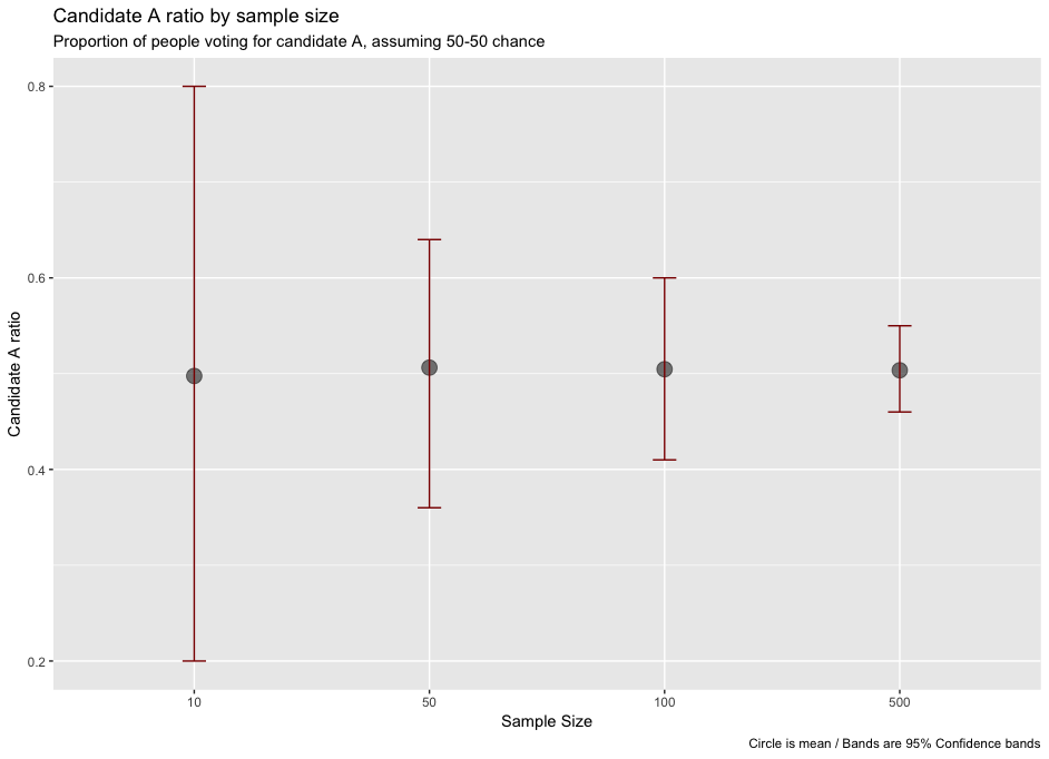
In this recipe, we have the number of people in a town, and whether they vote for Candidate A or Candidate B – these are flagged by 1s and 0s. We want to study the variability of several sample sizes, and ultimately we want to define which sample size is appropriate. Intuition would suggest that the error decreases nonlinearly as we increase the sample size: when the sample size is small, the error should decrease slowly as we increase the sample size. On the other hand, it should decrease quickly when the sample is large.

1. Import the libraries:

library(dplyr)
library(ggplot2)

2. Load the dataset:

voters_data = read.csv("./voters_.csv")

3. Take 1,000 samples of size 10 and calculate the proportion of people voting for Candidate A:

proportions_10sample = c()
for (q in 2:1000){
 sample_data = mean(sample(voters_data$Vote,10,replace = FALSE))
 proportions_10sample = c(proportions_10sample,sample_data)
}

4. Take 1,000 samples of size 50 and calculate the proportion of people voting for Candidate A:

proportions_50sample = c()
for (q in 2:1000){
 sample_data = mean(sample(voters_data$Vote,50,replace = FALSE))
 proportions_50sample = c(proportions_50sample,sample_data)
}

5. Take 1,000 samples of size 100 and calculate the proportion of people voting for Candidate A:

proportions_100sample = c()
for (q in 2:1000){
 sample_data = mean(sample(voters_data$Vote,100,replace = FALSE))
 proportions_100sample = c(proportions_100sample,sample_data)
}

6. Take 1,000 samples of size 500 and calculate the proportion of people voting for Candidate A:

proportions_500sample = c()
for (q in 2:1000){
 sample_data = mean(sample(voters_data$Vote,500,replace = FALSE))
 proportions_500sample = c(proportions_500sample,sample_data)
}

7. We combine all the DataFrames, and calculate the 2.5% and 97.5% quantiles:

joined_data50 = data.frame("sample_size"=50,"mean"=mean(proportions_50sample), "q2.5"=quantile(proportions_50sample,0.025),"q97.5"=quantile(proportions_50sample,0.975))
joined_data10 = data.frame("sample_size"=10,"mean"=mean(proportions_10sample), "q2.5"=quantile(proportions_10sample,0.025),"q97.5"=quantile(proportions_10sample,0.975))
joined_data100 = data.frame("sample_size"=100,"mean"=mean(proportions_100sample), "q2.5"=quantile(proportions_100sample,0.025),"q97.5"=quantile(proportions_100sample,0.975))
joined_data500 = data.frame("sample_size"=500,"mean"=mean(proportions_500sample), "q2.5"=quantile(proportions_500sample,0.025),"q97.5"=quantile(proportions_500sample,0.975))

8. After combining them, we use the Gaussian approximation to get the 2.5% and 97.5% quantiles. Note that we use 1.96, which is the associated 97.5% quantile (and -1.96 for the associated 2.5% quantile, due to the symmetry of the Gaussian distribution):

data_sim = rbind(joined_data10,joined_data50,joined_data100,joined_data500)
data_sim = data_sim %>% mutate(Nq2.5 = mean - 1.96*sqrt(mean*(1-mean)/sample_size),N97.5 = mean + 1.96*sqrt(mean*(1-mean)/sample_size))
data_sim$sample_size = as.factor(data_sim$sample_size)

9. Plot the previous DataFrame using the ggplot function:

ggplot(data_sim, aes(x=sample_size, y=mean, group=1)) +
 geom_point(aes(size=2), alpha=0.52) + theme(legend.position="none") +
 geom_errorbar(width=.1, aes(ymin=q2.5, ymax=q97.5), colour="darkred") + labs(x="Sample Size",y= "Candidate A ratio", title="Candidate A ratio by sample size", subtitle="Proportion of people voting for candidate A, assuming 50-50 chance", caption="Circle is mean / Bands are 95% Confidence bands")

This provides the following result:

We run several simulations, using different sample sizes. For each sample size, we take 1,000 samples and we get the mean, and 97.5% and 2.5% percentiles. We use them to construct a 95% confidence interval. It is evident that the greater the sample sizes are, the narrower these bands will be. We can see that when taking just 10 elements the bands are extremely wide, and they get narrower quite quickly when we jump to a larger sample size.

In the following table you can see why, when elections are tight (nearly 50% of voters choosing A), they are so difficult to predict. Since the election is won by whoever has the majority of the votes, and our confidence interval ranges from 0.45 to 0.55 (even when taking a sample size of 500 elements), we can't be certain of who the winner will be.

Take a look at the following results—95% intervals—left simulated ones; right Gaussian approximation: